Techniques for label conditioning in Gaussian denoising diffusion models

I go over some preliminaries here. If you're new to DDPMs, it may be best to read this first!

DDPMs can be derived by first starting off with the evidence lower bound, which can be expressed as:

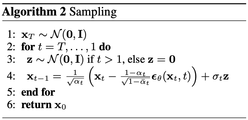
\begin{align} \label{eq:elbo} \log p(\xx) & \geq \text{ELBO}(\xx) \\ & = \mathbb{E}_{q(\xx_0, \dots, \xx_T)} \Big[ \underbrace{-\log \frac{p(\xx_T)}{q(\xx_T|\xx_0)}}_{L_T} - \sum_{t > 1} \underbrace{\log \frac{\pt(\xx_{t-1}|\xx_t)}{q(\xx_{t-1}|\xx_t, \xx_0)}}_{L_t} - \underbrace{\log \pt(\xx_0|\xx_1)}_{L_0} \Big. \tag{0} \end{align}

Using typical DDPM notation, \(\xx_0 \sim q(\xx_0)\) is the real data, and \(q(\xx_t|\xx_{t+1})\) for \(t \in \{1, \dots, T\}\) defines progressively noisier distributions (dictated by some noising schedule \(\beta_t\)), and \(\pt(\xx_{t-1}|\xx_t)\) parameterises a neural net which is trained to reverse this process. In practice, \(\pt\) is re-parameterised such that it in turn is a function of a noise predictor \(\epst(\xx_t, t)\) which is trained to predict only the noise in the image that is generated via \(\xx_t \sim q(\xx_t|\xx_0)\):

\begin{align} \pt(\xx_{t-1}|\xx_t) = \mathcal{N}(\xx_{t-1}; \frac{1}{\sqrt{\alpha_t}}\Big( \xx_t - \frac{1-\alpha_t}{\sqrt{1-\alphabar_t}} \epst(\xx_t, t)\Big), \sigma(\xx_t, t)). \end{align}

As a further simplification, each of the \(T\) KL terms in the ELBO can be simplified to the following noise prediction task:

\begin{align} \mathcal{L}(t) = \mathbb{E}_{\xx_0, \xx_t, \epsilon_t} \big[ \frac{\beta_t^2}{2\sigma_t^2 \alpha_t(1-\alphabar_t)} \| \epsilon_t - \epsilon_{\theta}(\xx_t, t)\|^{2} \big]. \end{align}

In practice, a biased version of the loss is used which removes the weighting term inside the square brackets. This has the effect of upweighting the loss in favour of noiser images (i.e. \(\xx_t\) for large \(t\)):

\begin{align} \mathcal{L}_{\text{simple}}(t) = \mathbb{E}_{\xx_0, \xx_t, \epsilon_t} \big[ \| \epsilon_t - \epsilon_{\theta}(\xx_t, t)\|^{2} \big]. \end{align}

The following derivations hinge on one important equation that relates diffusion models to score matching song2020score. I take the following from Lilian Weng's blog weng2021diffusion:

\begin{align} \st(\xx_t, t) \approx \nabla_{\xx_t} \log q(\xx_t) = -\frac{\epst(\xx_t, t)}{\sqrt{1 - \alphabar_{t}}}. \tag{1} \end{align}

The question we would like to answer in the following sections is: given an unconditional diffusion model \(\pt(\xx)\), how can we easily derive a conditional variant \(\pt(\xx|\yy)\)?

Through Bayes' rule we know that:

\begin{align} q(\xx_t|y) = \frac{q(\xx_t, y)}{q(y)} = \frac{q(y|\xx_t)q(\xx_t)}{q(y)}. \end{align}

Taking the score \(\nabla_{\xx_t} \log q(\xx_t|y)\), we get:

\begin{align} \nabla_{\xx_t} \log q(\xx_t|y) & = \nabla_{\xx_t} \log q(y|\xx_t) + \nabla_{\xx_t} \log q(\xx_t) - \underbrace{\nabla_{\xx_t} \log q(\yy)}_{= 0} \\ & \approx \nabla_{\xx_t} \log q(\yy|\xx_t) - \frac{\epst(\xx_t, t)}{\sqrt{1-\alphabar_t}}, \ \ \text{(using eqn. (1))} \tag{2a} \end{align}

where in the last line we make clear the connection between the score function and the noise predictor \(\epst\) weng2021diffusion. We could also use Equation (1) to do the same thing to the LHS of Equation (2a):

\begin{align} \nabla_{\xx_t} \log q(\xx_t|y) & \approx \nabla_{\xx_t} \log q(\yy|\xx_t) - \frac{\epst(\xx_t, t)}{\sqrt{1-\alphabar_t}} \\ \implies -\frac{\epst(\xx_t, \yy, t)}{\sqrt{1-\alphabar_t}} & \approx \nabla_{\xx_t} \log q(\yy|\xx_t) - \frac{\epst(\xx_t, t)}{\sqrt{1-\alphabar_t}} \tag{2b} \end{align}

If we re-arrange for \(\epst(\xx_t, \yy, t)\) in Equation (2b) we finally get:

\begin{align} \epst(\xx_t, y, t) & \approx \epst(\xx_t, t) - \sqrt{1-\alphabar_t} \nabla_{\xx_t} \log q(\yy|\xx_t) \tag{2c} \end{align}

The only thing left to do is to approximate the ground truth classifier \(q(\yy|\xx_t)\) with our own classifier \(\pphi(\yy|\xx_t; t)\). This will be defined as:

\begin{align} \epstt(\xx_t, y, t) := \epst(\xx_t, t) - \sqrt{1-\alphabar_t} \nabla_{\xx_t} \log \pphi(\yy|\xx_t; t). \tag{2d} \end{align}

This classifier should be trained on the same distribution of images from the forward process \(q(\xx_0, \dots, \xx_T)\) so that appropriate gradients are obtained during sampling. Note that I have also conditioned on \(t\) as well, which I suspect probably is a good extra supervisory signal so that the classifier knows what timestep \(\xx_t\) is coming from.

In practice, we can also define the weighted version as follows, which allows us to balance between (conditional) sample quality and sample diversity:

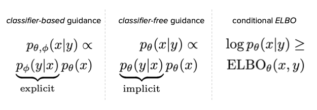
\begin{align} \label{eq:cg_supp} \underbrace{\bar{\epstt}(\xx_t, t, y; w) := \epst(\xx_t, t) -\sqrt{1-\bar{\alpha}_t} w \nabla_{\xx_t} \log \pphi(y|\xx_t; t)}_{\text{classifier-free guidance, plug this into Fig. 1}}. \tag{2e} \end{align}

Even though this form of label conditioning requires an external classifier, it is quite a simple and principled derivation, and therefore I like it. Essentially, from an unconditional diffusion model \(\pt(\xx)\) we are inducing a conditional variant at generation time. One can think of sampling from this particular noise predictor as sampling an \(\xx \sim p_{\theta,\phi}(\xx|\yy) \propto \pphi(\yy|\xx)\pt(\xx)\) for a given \(\yy\).

I think one interesting aspect of this formulation is that, since the induced conditional model is a function of both the unconditional model \(\pt(\xx)\) and the classifier \(\pphi(\yy|\xx)\), the entire generative model could be improved by switching out either component in isolation with an updated version. This could be useful if:

• it is too expensive to re-train the diffusion model at regular intervals. Since classifiers are a bit faster to train, one strategy could be to update (retrain) the classifier at more frequent intervals than the diffusion model.
• One wishes to leverage a pre-trained + frozen unconditional diffusion model for transfer learning with their own prescribed classifier.

The idea behind classifier-free guidance is that one could simply instead condition on \(\yy\) in the reverse process, i.e. use \(\pt(\xx_{t-1}|\xx_{t}, y)\) instead of \(\pt(\xx_{t-1}|\xx_t)\). In our case, this would be conditioning on \(\yy\) for the noise predictor \(\epst(\xx_t, y, t)\). However, the authors also propose learning the unconditional version at the same time for the same model, which means that during training \(\yy\) random gets dropped with some probability \(\puncond\). When the label does get dropped, it simply gets replaced with some null token, so we can think of \(\epst(\xx_t, t) = \epst(\xx_t, y = \emptyset, t)\). (In practice, dhariwal2021diffusion found that a \(\puncond\) of 0.1 or 0.2 works well.)

The reason for this algorithm is so that a variant of Equation (2c) can be derived without depending on an external classifier. From Bayes' rule, we know that:

\begin{align} \pt(\yy|\xx_t) = \frac{\pt(\yy,\xx_t)}{\pt(\xx_t)} = \frac{\pt(\xx_t|y)p(\yy)}{\pt(\xx_t)}, \end{align}

and that therefore the score \(\nabla_{\xx_t} \log \pt(\yy|\xx_t)\) is:

\begin{align} \nabla_{\xx_t} \log \pt(y|\xx_t)= \nabla_{\xx_t} \log \pt(\xx_t|y) + \underbrace{\nabla_{\xx_t} \log p(\yy)}_{= 0} - \nabla_{\xx_t} \log \pt(\xx_t). \end{align}

We simply plug this into Equation (2c) (as well as re-introduce \(w\)) to remove the dependence on \(q(y|\xx_t)\):

\begin{align} \bar{\epst}(\xx_t, y, t; w) & := \epst(\xx_t, t) -\sqrt{1-\bar{\alpha}_t} w \nabla_{\xx_t} \log \pt(y|\xx_t) \\ & = \epst(\xx_t, t) -\sqrt{1-\bar{\alpha}_t} w \Big[ \nabla_{\xx_t} \log \pt(\xx_t|y) - \nabla_{\xx_t} \log \pt(\xx_t) \Big] \\ & = \epst(\xx_t, t) -\sqrt{1-\bar{\alpha}_t} w \Big[ \frac{-1}{\sqrt{1-\bar{\alpha}_t}} \epst(\xx_t, y, t) - \frac{-1}{\sqrt{1-\bar{\alpha}_t}} \epst(\xx_t, t) \Big] \\ & = \epst(\xx_t, t) + w \epst(\xx_t, y, t) - w \epst(\xx_t, t) \\ & = \underbrace{\epst(\xx_t, t)}_{\approx \nabla_{\xx_t} \log p(\xx)} + w \Big( \underbrace{\epst(\xx_t, y, t) - \epst(\xx_t, t)}_{\approx \nabla_{\xx_t} \log p(\yy|\xx)} \Big). \tag{3a} \end{align}

From Equation (3a) we can see that the term being multiplied by \(w\) is (roughly) the score induced by the implicit classifier that defined by the diffusion model itself. Note that Equation (3a) could also be re-written as:

\begin{align} \underbrace{\bar{\epst}(\xx_t, y, t; w) := (1-w)\epst(\xx_t, t) + w \epst(\xx_t, y, t)}_{\text{classifier-free guidance, plug this into Fig. 1}}, \tag{3b} \end{align}

The previous two methods involve turning an unconditional diffusion model into a conditional one by either leveraging an explicit classifier (classifier guidance) or deriving an implicit one (classifier-free guidance). For the classifier-guided variant, the new conditional model can be written as:

\begin{align} p_{\theta,\phi}(\xx|\yy; w) & \propto \underbrace{\pphi(\yy|\xx)^{w}}_{\text{explicit}} \pt(\xx). \end{align}

For classifier-free, this classifier is implicit, and the balance between the two following terms isn't just via \(w\) at generation time but also through the training hyperparameter \(\puncond\):

\begin{align} \pt(\xx|\yy; w) & \propto \underbrace{\pt(\yy|\xx)^{w}}_{\text{implicit}} \pt(\xx). \end{align}

When we compare both formulations in this manner, we might also ask ourselves, what's stopping us from just training a conditional model \(\pt(\xx|\yy)\) directly, rather than through the product of a classifier and an unconditional model? This is certainly possible, via the conditional ELBO. This would correspond to taking Equation (0) and adding \(\yy\) to each conditional distribution, as well as converting the prior \(p(\xx_T)\) to a learned conditional prior \(\pt(\xx_T|\yy)\):

\begin{align} \log p(\xx|\yy) & \geq \text{ELBO}(\xx, \yy) \\ & = \mathbb{E}_{q(\xx_0, \dots, \xx_T, \yy)} \Big[ \underbrace{-\log \frac{\pt(\xx_T|\yy)}{q(\xx_T|\xx_0,\yy)}}_{L_T} - \sum_{t > 1} \underbrace{\log \frac{\pt(\xx_{t-1}|\xx_t,\yy)}{q(\xx_{t-1}|\xx_t, \xx_0, \yy)}}_{L_t} \\ & - \underbrace{\log \pt(\xx_0|\xx_1, \yy)}_{L_0} \Big]. \tag{4} \end{align}

To me, this is the most theoretically rigorous way to derive a conditional diffusion model. (In fact, this has already been used in lu2022conditional for speech diffusion!) Oddly enough, this doesn't appear to be the way that labelling is done in practice. Ironically, in the variational autoencoder literature this is how almost all conditional variants are derived, and diffusion models are just multi-latent generalisations of VAEs which learn \(T\) latent codes instead (with the added constraint that the dimensionality of those codes are the same as the input dimensionality). I suspect this is probably because, unlike in the case of VAEs, one has to think carefully about how \(\yy\) can be conditioned on in the forward process, especially if \(\yy\) is not the same dimension as \(\xx\).

For more details about this kind of model, I highly recommend you read my other post where I talk about lu2022conditional and implement a proof-of-concept that also works on discrete labels (through MNIST). I also show that one of the hyperparameters used in the training of this model also acts like a sort of knob that allows one to control between sample quality and diversity.

I will summarise everything with some key bullet points:

• Classifier-based / classifer-free guidance allow us to imbue unconditional diffusion models with the ability to condition on a label.
• Classifier-based guidance requires an external classifier, but decomposing the model into two modules may be beneficial from the point of view of retraining or fine-tuning on new data.
• Classifier-free guidance does not require an external classifier, but requires an extra hyperparameter \(\puncond\) during training. Since the same weights are used to parameterise both the implicit classifier and unconditional score estimator, it may be useful in a semi-supervised learning scenario.
• A more theoretically direct approach to conditioning on labels is to derive a Gaussian DDPM via the conditional ELBO (Equation (4)), but would require some extra derivations and model assumptions to be made. A conditional ELBO-based approach is used in lu2022conditional, and I speak about it here.
• All three variants allow for weighting trading off between sample quality and diversity.

• ho2020denoising Ho, J., Jain, A., & Abbeel, P. (2020). Denoising diffusion probabilistic models. Advances in Neural Information Processing Systems, 33(), 6840–6851.
• song2020score Song, Y., Sohl-Dickstein, J., Kingma, D. P., Kumar, A., Ermon, S., & Poole, B. (2020). Score-based generative modeling through stochastic differential equations. arXiv preprint arXiv:2011.13456, (), .
• classifierfree Ho, J., & Salimans, T. (2022). Classifier-free diffusion guidance. arXiv preprint arXiv:2207.12598, (), .
• dhariwal2021diffusion Dhariwal, P., & Nichol, A. (2021). Diffusion models beat GANs on image synthesis. Advances in Neural Information Processing Systems, 34(), 8780–8794.
• lu2022conditional Lu, Y., Wang, Z., Watanabe, S., Richard, A., Yu, C., & Tsao, Y. (2022). Conditional diffusion probabilistic model for speech enhancement. In , ICASSP 2022-2022 IEEE International Conference on Acoustics, Speech and Signal Processing (ICASSP) (pp. 7402–7406).
• weng2021diffusion Weng, L. (2021). What are diffusion models? lilianweng.github.io, (), .
• sohn2015learning Sohn, K., Lee, H., & Yan, X. (2015). Learning structured output representation using deep conditional generative models. Advances in neural information processing systems, 28(), .