\(\newcommand{\xx}{\boldsymbol{x}}\) \(\newcommand{\yy}{\boldsymbol{y}}\) \(\newcommand{\pt}{p_{\theta}}\) \(\newcommand{\QQ}{\boldsymbol{Q}}\) \(\newcommand{\mm}{\boldsymbol{m}}\) \(\newcommand{\alphabar}{\bar{\alpha}}\) \(\newcommand{\mt}{\mu_{\theta}}\) \(\newcommand{\epst}{\epsilon_{\theta}}\) \(\newcommand{\betatilde}{\tilde{\beta}}\) \(\newcommand{\deltatilde}{\tilde{\delta}}\) \(\newcommand{\linspace}{\text{linspace}}\) \(\newcommand{\embed}{\text{embed}_{\theta}}\)
Learning the conditional prior over classes for image diffusion
If you found this useful and wish to cite it, you can use this corresponding Bibtex entry:
@misc{beckham2022_condprior,
  author = {Beckham, Christopher},
  title = {Tech report: Learning the conditional prior over classes for image diffusion},
  year = {2022},
  howpublished = {\url{https://beckham.nz/2022/09/24/cond-diffusion.html}}
}
The Github repository for this code can be found here.
Table of contents
Unconditional diffusion
Let us start with a quick refresher for a typical (unconditional) diffusion model (see [1] for more details). The \(t\)-step forward process can conveniently be derived to give us the following:
\begin{align} \label{eq:uncond_fwd_t_step} q(\xx_t|\xx_0) = \mathcal{N}(\xx_t; \sqrt{\alphabar_{t}}\xx_0, (1-\alphabar_{t}) \mathbf{I}) \end{align}
The reverse process can be formulated as:
\begin{align} \label{eq:uncond_reverse} \pt(\xx_{t-1}|\xx_t) = \mathcal{N}(\xx_{t-1}; \mt(\xx_t, t), \betatilde_t \mathbf{I} ) \end{align}
where:
- \(\betatilde_t = \frac{1-\alphabar_{t-1}}{1 - \alphabar_{t}} \beta_t\);
- \(\mt(\xx_t, t) = \frac{1}{\sqrt{\alpha_t}} \xx_t - \frac{\beta_t}{\sqrt{\alpha_t} \sqrt{1-\alphabar_{t}}}\epst(\xx_{t}, t)\); that is, we parameterise a neural network that tries to predict the noise.
The conditional variant
In this report I consider the paper proposed by [2], which proposes a conditional variant of diffusion for speech synthesis. It’s presented as a very principled derivation, in the sense that their formulation can be seen as a generalisation of unconditional diffusion. The formulation is a bit math heavy, and I will simply defer you to their work if you want more details. Essentially, in their formulation \(\yy\) is actually ‘noisy’ version of \(\xx\) rather than a discrete label, so it presents itself as being a conditional diffusion model that can map between two domains (clean vs noisy speech). However, soon I will explore modifying this formulation so that one can instead condition on a discrete label.
Instead of deriving the one-step (conditional) forward first \(q(\xx_t | \xx_{t-1}, \yy)\) and then subsequently deriving \(q(\xx_t | \xx_{0}, \yy)\), the authors take the opposite approach and derive first \(q(\xx_t | \xx_{0}, \yy)\):
\begin{align} q(\xx_t | \xx_0, \yy) = \mathcal{N}(\xx_t; (1-\mm_t) \sqrt{\alphabar_{t}} \xx_0 + \mm_t \sqrt{\alphabar_{t}} \yy, \delta_{t} \mathbf{I}) \nonumber \end{align}
where the mean is characterised by a convex combination between the two terms, with \(\mm_t \in [0,1]\) being the interpolation coefficient. Essentially, as we run the forward diffusion, the mean progressively moves towards a scaled \(\yy\) under some variance schedule \(\delta_t\). Because of the interpolation, we can see that \(\yy\) must be of the same dimensionality as \(\xx\) as well. The prior distribution for some \(\yy\) can be expressed as:
\begin{align} \pt(\xx_T |\yy) = \mathcal{N}(\xx_T; \sqrt{\alphabar_T} \yy, \delta_{T} \mathbf{I}) \nonumber \end{align}
so that \(\yy\) essentially parameterises the mean of the conditional prior \(\pt(\xx_T|\yy)\)
up to the scaling factor \(\sqrt{\alphabar_T}\).
From which they show that under a particular derivation for \(\delta_t\), marginalising \(q(\xx_t|\xx_0,\yy)\) over \(\yy\) recovers the unconditional forward process \(q(\xx_t|\xx_0)\):
\begin{align} \delta_t = (1 - \alphabar_{t}) - m_t^2 \alphabar_t \nonumber \end{align}
hence this is a conditional generalisation of forward diffusion. \(\delta_t\) here is analogous to the \(\beta_t\) in the unconditional version. After some crazy long derivations, the authors derive the reverse process. This takes in a similarly convenient form, which is basically:
\begin{align} \label{eq:cond_reverse} \pt(\xx_{t-1}|\xx_{t}, \yy) = \mathcal{N}(\xx_{t-1}; \mt(\xx_t, \yy, t), \deltatilde_{t} \mathbf{I} ) \nonumber \end{align}
where:
- \(\deltatilde_t = \frac{\delta_{t|t-1} \cdot \delta_t}{\delta_{t-1}}\) (analogous to \(\betatilde_t\) in the unconditional version of the learned reverse process)
- \(\delta_{t|t-1} = \delta_{t} \Big( \frac{1 - m_t}{1 - m_{t-1}} \Big)^{2} \alpha_{t} \delta_{t-1}\) (this is also the variance term of \(q(\xx_t | \xx_{t-1}, \yy)\), so its analogue in the unconditional \(q(\xx_t | \xx_{t-1})\) would be \(\beta\))
Reproduction
I had issues with trying to get this to work on images. The paper didn’t go into details about how the ‘noisy’ \(\yy\) is constructed, apart from some comments that this is produced by interpolating different audio signals to corrupt the original \(\xx\). There were two strategies I conceived:
- (1) generate a noisy \(\yy\) via some interpolation \(\yy = \lambda \xx + (1-\lambda)\boldsymbol{\epsilon}\) where \(\lambda\) is sampled from some distribution whose support is in \([0,1]\) and \(\epsilon \sim \mathcal{N}(0, \mathbf{I})\). For instance, we could define \(\lambda \sim \text{Uniform}(a,b)\) for some hyperparameters \(a\) and \(b\) (this is also called mixup [3]).
- (2) learn an embedding for \(\yy\). Essentially, let \(y'\) denote the \emph{actual label} of the image, and let \(\yy = \text{embed}_{\theta}(y')\) be a learnable embedding layer that maps a label to a tensor of the same dimensions as the original image, whose parameters will also be updated in unison with those from the noise predictor \(\epst\) (hence the subscript \(\theta\)). This formulation therefore requires a modification to Algorithms 1 and 2 in the original paper.
I initially tried (1) but found results vary quite a bit depending on \(\yy\). If it is too close to the original image then you recover it, if it’s too high then you either get bad looking images or you get the same images every time (as if the noise does not matter). For (2) I just ended up getting mode dropping in general.
For this I decided to go with (2), since (1) is more akin to a domain translation type of problem and I want to do conditional generation in the more general sense (conditioned on a discrete label or token). What I found solved it was to carefully consider the schedule for $\mm$. The original paper set \(\mm\) to:
\begin{align} \mm_t = \sqrt{ (1-\alphabar_{t}) / \sqrt{\alphabar_t}} \nonumber \end{align}
and remark that it gives \(\mm_0 = 0\) and \(\mm_T \approx 1\), but this only holds for a specific parameterisation of \(\beta_t\). in particular the two choices of \(\beta\) that were chosen for the experiments in [2]:
- Base CDiffuSE: \(\beta_t \in [1 \times 10^{-4}, 0.035]\)
- Large CDiffuSE: \(\beta_t \in [1 \times 10^{-4}, 0.0095]\)
Of course, one could enforce \(\mm\) to be within this range by setting \(\mm\) to be something like \(\linspace(0, 1, T)\), but I found that changing this did not make a difference when it came to getting my experiments working. In fact, setting \(\mm = \text{linspace}(0, \tau, T)\) seemed to resolve this, for some ‘reasonable’ values of \(\tau\). Note that \(\mm_{T} = \tau\). In Figure 1 we can see randomly generated images for different values of \(\tau\), after 10 epochs of training with a \(\beta_{t} \in [0.0001, 0.02]\) (these are just defaults I inherited from the original difusion code). It appears that if \(\tau\) is too ‘large’ (close to one) then samples exhibit low diversity, yet when \(\tau\) is too small (close to zero) samples are not as likely to be as class consistent (i.e. reflect the label it was conditioned on). In general:
\begin{align} \pt(\xx_T | \yy) = \mathcal{N}(\xx_T; \tau \sqrt{\alphabar_T} \yy, \delta_{T} \mathbf{I}), \nonumber \tag{1} , \end{align}
so it seems like when \(\tau\) is too small then the magnitude of the mean in \(\xx_T \sim \pt(\xx_T|\yy)\) (which is a function of \(\yy\)) becomes diminished. When \(\tau\) is too large, I hypothesis that maybe this is because the variance schedule becomes too large (see Figure 1).
Examining different values of \(\tau\)
| $$\tau=0.3$$ | $$\tau=0.5$$ | $$\tau=0.7$$ |
|---|---|---|
 |
 |
|
| $$\tau= 0.8$$ | $$\tau= 0.9$$ | $$\tau = 1.0$$ |
|---|---|---|
 |
 |
 |
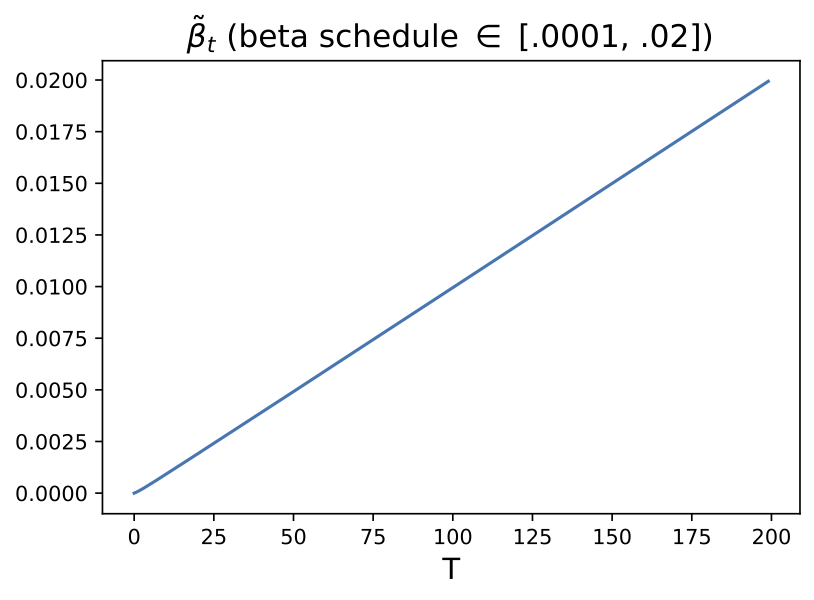
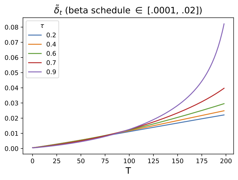
Since \(\tilde{\delta_t}\) is the conditional analogue to \(\tilde{\beta}\) (and that \(\tilde{\delta_t}\) is also a function of \(\mm\)), we plot these two variables to see how the variance changes as a function of time. This is shown in Figure 2.
Reverse diffusion
Using \(\tau = 0.7\), we can visualise the reverse difffusion for ten randomly sampled images per class, for a grid of 100 generated examples in total.
For the sake of time I have simply chosen to visualise what qualitatively looks to be the best \(\tau\); however in practice we should select the one which gives us the best FID or likelihood on the data.
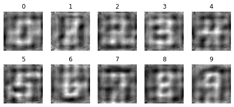
Visualising the learned embeddings
What is interesting is that we can visualise the learned y’s by the network; these are what we start off with when we run the learned reverse diffusion as described in Equation (1). In Figure 3 we visualise the learned embeddings \(\yy = \embed(y')\) for \(y' \in \{0, 1, \dots, 9\}\). We can see that the network has, in a sense, learned ‘pseudo examples’ that parameterise the mean of \(p(\xx_T|\yy)\) for each of the classes.
If I can shamelessly plug my own work here, in [4] we proposed a way to ‘incrementally’ fine-tune a generative model simply by adding the new classes’ indices to the lookup table that is the embedding layer. Surely, a similar thing could be done here (assuming that our diffusion model is ‘expressive’ enough to facilitate generating from these new classes).
References
- [1] Ho, J., Jain, A., & Abbeel, P. (2020). Denoising diffusion probabilistic models. Advances in Neural Information Processing Systems, 33, 6840-6851.
- [2] Lu, Y. J., Wang, Z. Q., Watanabe, S., Richard, A., Yu, C., & Tsao, Y. (2022, May). Conditional diffusion probabilistic model for speech enhancement. In ICASSP 2022-2022 IEEE International Conference on Acoustics, Speech and Signal Processing (ICASSP) (pp. 7402-7406). IEEE.
- [3] Zhang, H., Cisse, M., Dauphin, Y. N., & Lopez-Paz, D. (2017). mixup: Beyond empirical risk minimization. arXiv preprint arXiv:1710.09412.
- [4] Beckham, C., Laradji, I., Rodriguez, P., Vazquez, D., Nowrouzezahrai, D., & Pal, C. (2022). Overcoming challenges in leveraging GANs for few-shot data augmentation. arXiv preprint arXiv:2203.16662.