reflecting on past work -- offline model-based optimisation

Table of Contents
In this post, I introduce offline model-based optimisation and share some highlights from research I published at the tail end of my PhD [1]. The focus is on issues of validation and extrapolation – two topics that remain frustratingly underexplored in the field. Along the way, I offer an honest critique of my own work, reflect on broader challenges in offline MBO, and point to a few promising directions forward.
While I’m no longer working in academia, this topic still matters a lot to me. If any of it resonates with you – whether you’re a researcher, engineer, or just curious, I’d love to chat, albeit in a bandwidth-conscious capacity.
1. intro - what is model-based optimisation?
In model-based optimization (MBO), the goal is to design inputs—often tangible, real-world objects—that maximise a reward function reflecting some desired property. Crucially, this reward function exists in the real world, meaning that evaluating it requires physically testing the input and observing its outcome. For example, in protein design, the input might be a molecular specification, and the reward could be the protein’s ability to bind to a specific kind of receptor in the body. In this setting, the true objective \(f(x) \in \mathbb{R}^{+}\) measures binding affinity, and querying it involves running expensive lab experiments. We will refer to this "true" objective function as the reward oracle.
In theory, we could optimise the reward oracle \(f\) directly by combining it with a search algorithm, learning from past evaluations to guide the search for better inputs. This involves learning a "surrogate" model \(\ft\), which is exploited by the search algorithm and is also refined iteratively based on feedback provided by the reward oracle. This is called online model-based optimisation ("online MBO"). In practice however, querying \(f\) is often prohibitively expensive and slow, and we need many samples if we want the surrogate model to learn enough about the underlying problem in order to guide the search towards promising candidates.
But if we already have an existing dataset of input-reward pairs (here \(y = f(x)\) is the "reward"), we can use it to pre-train the surrogate model. The idea is that a well-trained surrogate may then require far fewer queries during the online phase to guide the search effectively. This pre-training stage is known as offline model-based optimisation ("offline MBO").
Since \(\ft\) is an approximation however, it is particularly brittle. It can behave unpredictably on regions of input space which are not represented in the training data (what we call "out-of-distribution"), and this is especially problematic since we assume the best input candidates are not already yet in the training set. Such models are also vulernable to "adversarial examples", where by naively optimising for the highest-scoring candidate with respect to the surrogate often produces one which is no longer plausible according to real world constraints. This makes it an interesting yet challenging area of research.
1.1. formalising offline mbo
In the offline setting, we assume access to a labelled dataset of input-output pairs, denoted \(\mathcal{D} = \{(x_i,y_i)\}_{i=1}^{N}\), where \(y_i \in \mathbb{R}^{+}\) and \(y_i = f(x_i)\). The goal is to learn a model of the reward – typically a surrogate function \(\ft\) – without querying the true function during training or model selection. While much of the offline literature focuses on a surrogate \(\ft\), it's arguably more useful to think in terms of a generative model that defines a joint distribution \(\pt(x,y)\). Via Bayes' rule, it can factorise in one of two ways.
The first is \(\pt(y|x)p(x)\), and we can think of \(\pt(y|x)\) as the probabilistic form of the surrogate, i.e. \(\ft(x)\) parameterises the mean of the distribution. We can interpret this as: first we sample \(x\) from some prior (e.g. the training distribution), then we predict its reward. While this is technically a generative model, it is not particularly useful for sampling high-scoring candidates as the only sampling we do is from the training data (and not a model we have learned).
In practice, a common baseline takes a hybrid approach which doesn't quite correspond cleanly to this. This involves sampling \(x\) from the training data \(x \sim \ptrain(x)\), which is then iteratively updated by ascending the gradient of \(\ft(x)\) (which is typically the mean of \(\pt(y|x)\)). While this produces inputs with higher predicted reward, it abandons the semantics of the above factorisation and tends to produce poor inputs when scored against the reward oracle.1
The second factorisation is \(\pt(x|y)p(y)\), which we can think of as saying: first choose the desired reward \(y\), then find an input which has that reward. Since \(\pt(x|y)\) is a conditional generative model, not only can we target high reward regions, we can also avoid generating implausible inputs since it is a mechanism built into the model. (While generative models are not totally invulnerable to generating implausible inputs, they still do a lot better than discriminative models as plausibility is built into the model by design, i.e. likelihood.)
For the remainder of this work, we will define our joint generative model \(\pt(x,y)\) as the second factorisation:
\begin{align} \pt(x,y) = \pt(x|y)\ptrain(y), \end{align}where \(\ptrain(y)\) is the empirical distribution over the rewards in the training set.
1.2. reward-based extrapolation
The key idea which seperates MBO from regular generative modelling is that we don't just want to generate any kind of sample from the model. We would like to generate samples whose real reward \(y\) is as large as possible, as these have the most real world utility. The difficulty lies in the fact that these (extremely) high scoring samples do not exist in the training set, otherwise MBO would be a much simpler task where we only need to generate things that plausibly look like what is already in the training set. This means MBO has to extrapolate – it has to learn what constitutes low and medium-scoring samples, and infer what a high-scoring sample may look like.
This also implies that the behaviour of the generative model needs to somehow be "tweaked" at generation time. For instance, we have defined a generative model \(\pt(x,y)\) to be the following:
\begin{align} \pt(x,y) = \pt(x|y)\ptrain(y), \end{align}where \(\ptrain\) is the empirical distribution of \(y\)'s observed in training. If we simply sample according to this strategy, we will only sample conditioned on the kinds of reward seen in the training set. To rectify this, we could switch out the prior for another distribution \(\widehat{p}(y)\), one which reflects a larger distribution of rewards. For instance, if \(\ptrain(y)\) reflects a range of values from \([0,100)\), perhaps the new prior reflects those from \([100,200]\). From this, we can define the "extrapolated" model:
\begin{align} \widehat{\pt}(x,y) = \pt(x|y)\widehat{p}(y). \end{align}(I am using the widehat notation '\(\widehat{\pt}\)' to symbolise 'higher', a version of \(\pt\) which is biased towards high scoring samples, rather than something implying a statistical approximation.)
Ideally we would like to find an "extrapolated" model \(\widehat{\pt}(x,y)\) such that it maximises the average reward coming from the reward oracle, which we will simply call the "test reward":
\begin{align} m_{\text{test-reward}}(\tilde{p}) = \mathbb{E}_{x \sim \tilde{p}(x,y)} f(x), \tag{1} \end{align}and therefore we wish to maximise \(m_{\text{test-reward}}(\ptnew)\). In other words, we want to find a \(\pt(x|y)\) and \(\widehat{p}(y)\) such that samples produced by the former have as large of a reward as possible, according to the reward oracle. Since this equation involves \(f\) which is too expensive to compute during training or model selection, it is only intended to be executed at the very end of the machine learning pipeline. But this does not help us during training or model selection.
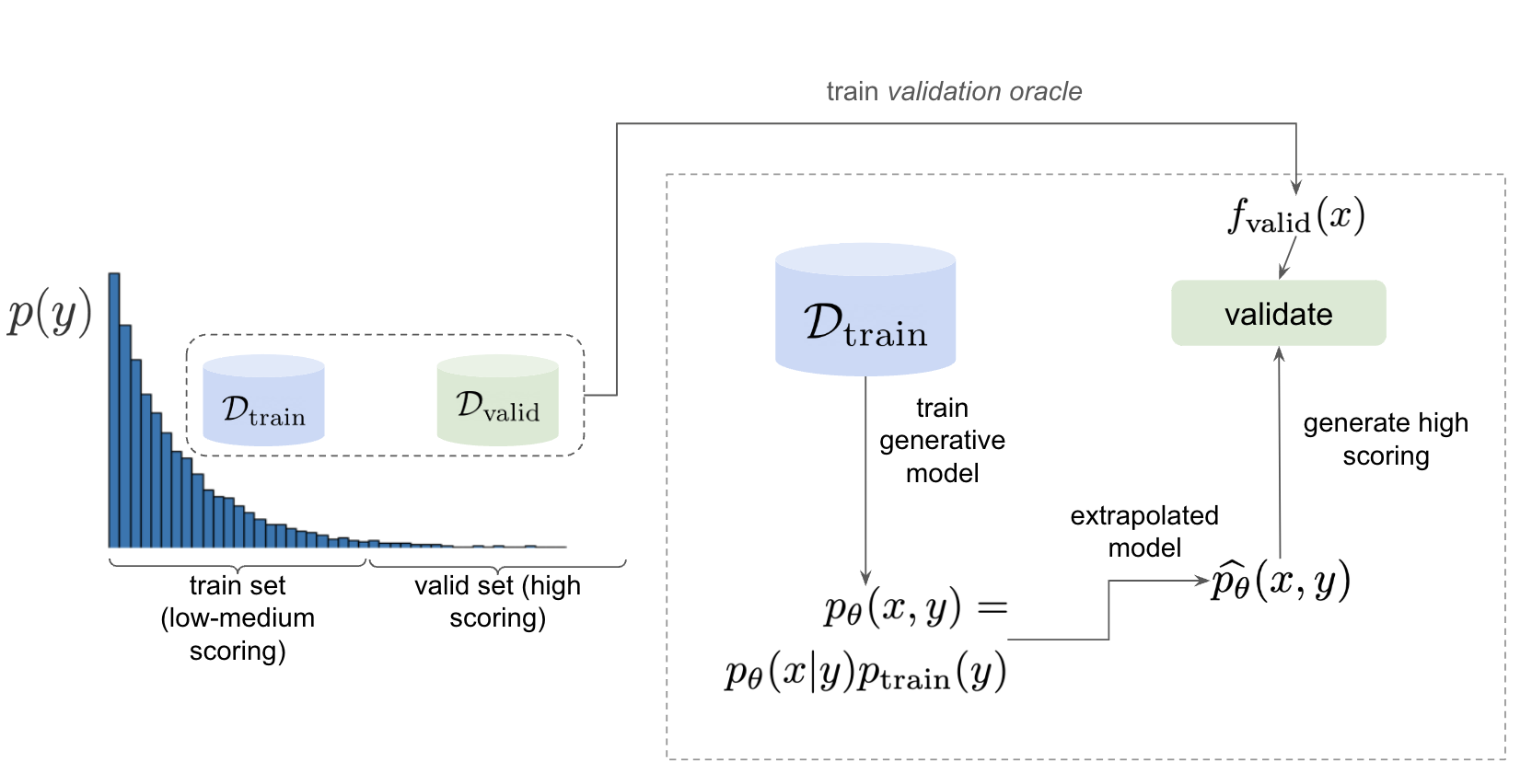
To rectify this, we could simply replace \(f\) with the surrogate model \(\ft\). However, \(\ft\) has also only been trained on the same empirical distribution of rewards, and we cannot expect it to score inputs conditioned on e.g. \([100,200]\) reliably, as this is clearly out-of-distribution. One approach is to split the dataset into low-to-moderate scoring examples and high-scoring examples. For instance, if our original dataset only represented samples with reward in \([0,100]\), then we could for instance split it into \([0,50]\) (low-to-moderate) and \([50,100]\) for high scoring (see Fig. 1). The low-to-moderate split is used to train the generative model, while the latter forms a validation set.
Both data splits (which is just the full dataset) can actually used to train a validation proxy, \(\fvalid\). It makes sense to evaluate \(\ptnew\) against this because it has been trained on the full distribution of rewards coming from the dataset. Since \(\fvalid\) has "seen" samples in \([50,100]\), even if the generative model hasn't, it can still produce inputs conditioned on this range and we can use the validation proxy to validate it. Therefore, this setup allows us to measure not just generalization, but generalization specifically in the context of reward extrapolation.
1.3. ‼️ why evaluation is difficult (and misunderstood)
With the rapid progress in generative modeling over the past few years, our approach to evaluation has evolved. In earlier eras of machine learning, it was common to assess models based on likelihood over a test or validation set – a natural outcome of maximum likelihood estimation, where the goal is to find parameters \(\theta\) that maximise the probability of the observed data.
Because of the extremely rapid advances in generative modelling in the past few years, the way we have performed evaluation has changed. In the olden days of machine learning, it was more common to evaluate machine learning models by way of likelihood on a test or validation set. This is a natural consequence of maximum likelihood estimation, which states that we wish to find a model which best "explains" the data, i.e. find parameters \(\theta\) such that the parameterised model assigns the highest average likelihood across all samples. However, likelihood is only concerned with how plausible pre-collected samples are, rather than whether samples generated from the model itself satisfy a useful notion of preference. (Also, likelihood isn't a particularly accurate measure of sample quality. [2], [3], [4]) Such preferences can be encoded with a reward function \(f\), but this is typically expensive to compute as it reflects a real world process (i.e. \(y = f(x)\) is like asking a human rater to evaluate \(x\)).
As mentioned in Sec. 1.2, a principled strategy is to approximate \(f\) with \(\fvalid\) and continue forward. Even if \(\fvalid\) is an approximation, it actually serves as a useful anchor for the generative model. This is because even though it is only trained on low-to-moderate scoring inputs, we can measure its ability to generate high-scoring inputs against the validation proxy which has technically seen high scoring inputs during training. Compared to other MBO literature, I make a very explicit distinction between validation and testing which does not seem to be well-respected, and I partly suspect it's because there is a conflation between "real world" MBO and "academic" MBO. (These are terms I created, and the latter is not meant to be read in a disparaging sense.)
By "academic MBO" I simply mean doing MBO in the context of academic research, i.e. publishing papers. In this situation it may not be practically feasible to evaluate the reward oracle \(f\), for instance in the case where the benchmark data involves an extremely expensive human evaluation (e.g. protein synthesis). To rectify this, some MBO datasets are actually based on simulation environments, and the same simulation provides a reward oracle which can be used to score the data.
Since the simulator is just a function that can be freely executed in silico with negligible monetary cost, researchers can (intentionally or not) "violate the spirit" of offline MBO by abusing the simulator and constantly querying it during training or model seleection.2 This is especially enticing in academia because there is an overwhelming bias towards pushing things that "beat SOTA" or are "novel". Conversely, in "real world" MBO there is already a safeguard against abusing the ground truth and that is time and money. Therefore, in order to respect the economic burden associated with MBO, a validation set needs to set aside as this is ultimately what we will use in the real world before sending off samples to be tested.
Apart from simulation environments, most MBO datasets are really just finite collections of data from a real world problem. Since the reward oracle is infeasible to compute for academic research, a "test proxy" \(\ftest\) is trained on the entire dataset and used as an approximation to the reward oracle. Like with the simulator, this can be easily abused, and necessitates the use of a seperate validation proxy \(\fvalid\).
Due to the different types of rewards oracles already mentioned, below is a table explaining what they are for:
| name | what is it |
|---|---|
| reward oracle | \(f(x)\): real world reward model, extremely expensive to compute. This may also refer to a simulation environment's reward model. |
| "proxy" oracle | - \(\ft\): a regression model trained on the training set. While it is a discriminative model, it can be "hacked" to act as a generative model. In this article, I prefer to use generative modelling terminology, in which case \(\pt(y \vert x)\) is used instead. However, in this post I prefer to use the conditional density \(\pt(x \vert y)\) will usually be referred to, instead of the other terms. |
| - \(\fvalid\) : typically not defined in literature, but this is specifically a proxy oracle intended for model selection and hyperparameter tuning. It is trained on the combined training and validation set. Here we will call it the validation proxy. | |
| - \(\ftest\) : proxy oracle trained on train + valid + test set (all of the data). This typically exists in "academic MBO" where the ground truth is also too impractical to compute at test time. Here we will call it the test proxy. |
1.4. training, validation, and testing
As discussed in Sec. 1.2, we need to measure not just generalisation, but extrapolation. If our validation set follows the proposed setup in Fig. (1), then we can just approximate Eqn. (1) by introducing some approximate reward model \(\tilde{f}\):
\begin{align} m_{\text{reward}}(\tilde{p}; \tilde{f}) &= \mathbb{E}_{x \sim \tilde{p}(x,y)} \tilde{f}(x). \tag{2} \end{align}From this, the function \(m_{\text{reward}}(\widehat{p_{\theta}}; \fvalid)\) now constitutes our first validation metric. By "validation metric" we simply mean some function which measures the ability of the model to extrapolate. More generally, it may not only be a function of an approximate oracle \(\tilde{f}\), but also other things such as the validation set itself. (We will discuss some other ones later.)
Note that while Eqn. (2) is a principled and reasonable approach to determining how well \(\pt(x|y)\) extrapolates, this is just one possible validation metric of many. On one hand, it is quite interpretable: assuming a fixed \(\fvalid\), Eqn. (2) is maximised when samples produced from \(x \sim \pt(x|y), y \sim \pvalid(y)\) produce the largest average reward. On the other hand, \(\fvalid\) is an approximate model and shares the same vulnerabilities to adversarial examples and overconfidence as many other regression model. Therefore, validation metrics go beyond Eqn. (2), and may involve measuring other aspects of the generative model or data.
So far we have discussed the need to measure extrapolation (Sec 1.2), as well as the lack of a validation set which is crucial to measuring it (Sec 1.3). From this we can motivate a very principled and reasonable train-validate-test recipe, which is the following:
- Inputs: Split total dataset \(\mathcal{D}\) into: \(\dtrain\), \(\dvalid\), and \(\dtest\). Ensure that the valid and test sets contain higher reward inputs, as per Sec. 1.2.
- Training: Train the generative model \(\pt(x|y)\) on \(\dtrain\). Also, if the validation metric necessitates it, train a validation proxy \(\fvalid\) on \(\dtrain \cup \dvalid\).
- Validation: Use \(\dvalid\) and/or \(\fvalid\) for model selection / hyperparameter tuning.
- Final evaluation: assuming we already have a recipe for generating high scoring samples from the model, score those samples with either the reward oracle (if we operate in "real world MBO"), or test proxy (if we operate in "academic MBO").
- If we need the test proxy, train a \(\ftest\) on \(\mathcal{D}\), and measure the average reward via \(m_{\text{reward}}(\widehat{p_{\theta}}; \ftest)\).
Finally: note that for the "real world MBO" step in "final evaluation", since we'll be sending off samples to the real world, it is much more data efficient to first re-train the best model on the entire dataset \(\mathcal{D}\) using the same hyperparameter configuration, and then use that to generate samples.
In the absence of a reward oracle which can be judiciously evaluated, we need to turn to cheap-to-compute validation metrics. We already saw one in Eqn. (2), and there are many others which can be conceived of. Given a list of these metrics a-priori, how can we figure out which one performs the best for our task?
2. last year's work
Let us begin with a summary of everything so far:
- (1) In offline model-based optimisation we wish to learn a reward-conditioned generative model from an offline dataset of input-reward pairs. The rewards are originally obtained from a ground truth reward "oracle", which is assumed to be too expensive to query during training or validation of the generative model.
- (2) Evaluating samples from a generative model is a difficult task. Firstly, likelihood-based evaluation is not sufficient to evaluate the quality of outputs. Secondly, samples ideally need to be evaluated by human feedback (which is perfectly encapsulated by the notion of a reward oracle). Lastly, models trained need to extrapolate beyond the rewards they were trained on, as the better they can extrapolate, the more impactful they will be in the real-world.
- (3) Evaluation is difficult, often neglecting a validation set. This may be related to the confusion between "real world" and "academic" MBO. In "academic MBO", the reward oracle is replaced with a test proxy or simulator. While these are technically useful and cheap-to-compute, non-sparing use of these fundamentally violate the spirit of offline MBO, whose emphasis is on trying to extract as much value as possible from the available data without resorting to expensive reward oracle queries.
- (4) (Repeating last section's paragraph) In the absence of a reward oracle which can be judiciously evaluated, we need to turn to cheap-to-compute validation metrics. We already saw one in Eqn. (2), and there are many others which can be conceived of. Given a list of these metrics a-priori, how can we figure out which one performs the best for our task?
The work I published last year addresses these points.
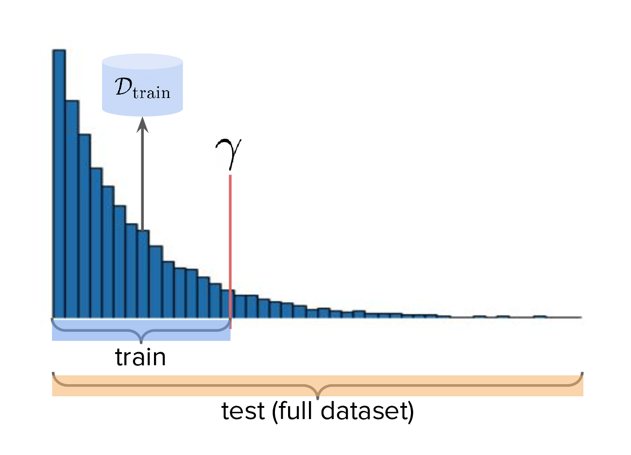
To implement the train-valid-test protocol described, some technical considerations were needed. Experiments were implemented with Design Bench, a popular MBO benchmarking framework [5]. Design Bench imposes a reward threshold \(\gamma\) which dictates which samples are assigned to the training set. For example, any samples whose \(y \leq \gamma\) are assigned to the training set, and the rest is obscured from the user (in an API-like sense). Because of this, all of the remaining samples \(\gt \gamma\) are not assigned to a validation set – in fact, the library does not prescribe one at all. Two possible solutions are:
- (1) Simply hold out some small part of the training set as the validation set. This respects the intended design of the library, but effectively reduces the size of the training set and therefore handicap model performance compared to other Design Bench-based models which use the full training set. (In Fig. 1 left, \(\dtrain\) is shown here, so imagine cutting out some portion of this as the validation set.)
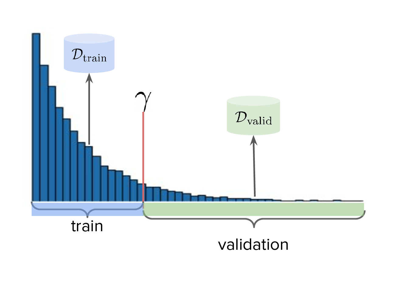
- (2) Define that all samples whose \(y \gt \gamma\) belong to the validation set (Fig. 1, right). Since the validation proxy \(\fvalid\) is always trained on the combined train+valid split, this means it is trained on the full dataset. This technique does not respect the intended design of the library, even if its motivation is quite principled.
I chose (2), which is illustrated in Fig. (3)-right. However, this requires some nuance when it comes to interpreting the relationship between the validation proxy \(\fvalid\) and the test oracle \(\ftest\). If the dataset is based on a simulator, then we already have "\(f\)" and we can train \(\fvalid\) on the full dataset as the simulator can be treated as the ground truth from which the dataset's samples were drawn from.
Otherwise, if \(\ftest\) is actually an approximate test oracle, then by Design Bench's definition it has been trained on the full dataset. This means training a validation proxy would involve training on all of the data and therefore be equivalent to a test oracle. But the latter needs to have seen more data to be a useful tool to measure generalisation once training and validation is completed. Therefore, in this situation, we let the test surrogate remain as the "gold standard" which has been trained on all of the data, and we only allow the validation proxy to be trained on a subset of the full dataset. Concretely, this would be the training set, plus an X% subsample of any examples whose reward exceeds \(\gamma\). This is shown below in Fig. (4), and in this illustration X% is 50%.
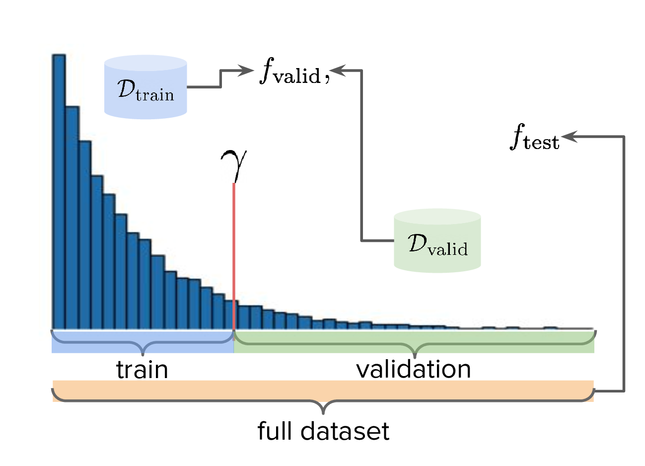
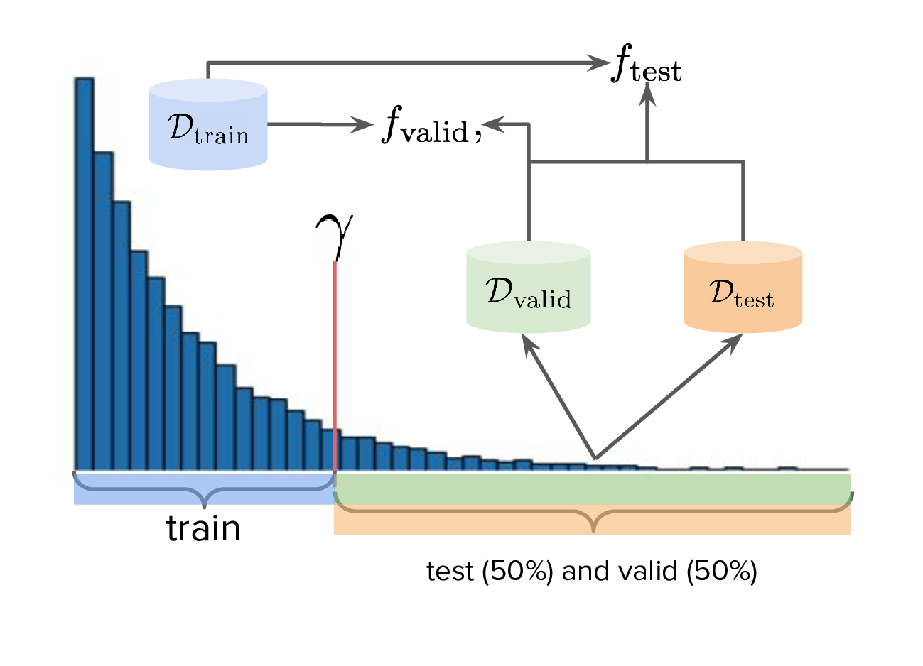
Therefore, for Design Bench, if we are dealing with a task for which no simulator environment exists, then we have to use a test proxy. That means invoking Fig. (4) for determining the precise train, valid, and test splits. Otherwise, if a simulator already exists, then we invoke Fig. (3).
2.1. ranking validation metrics
Now, all that is left is a validation metric. This metric is a function of the generative model \(\pt\), and may also be a function of the validation proxy \(\fvalid\) and validation set \(\dvalid\). (To keep notation light, we will assume that the metric \(m\) can take arbitrary number of arguments, even though so far we see it as a function of the first two.)
We already saw one of these metrics, which is simply Eqn. (2) but with \(\fvalid\) substituted for \(\tilde{f}\), which is just \(m_{\text{reward}}(\tilde{p}; \fvalid)\):
\begin{align} m_{\text{reward}}(\ptnew, \fvalid) & = \mathbb{E}_{x \sim \ptnew(x,y)} \fvalid(x) \\ & = \mathbb{E}_{x \sim \pt(x|y)\pvalid(y)} \fvalid(x). \tag{3} \end{align}This metric doesn't particularly care about how "calibrated" the model is. For instance, if we condition on \(y = 50\) and get an example whose reward according to \(\fvalid\) is \(1000\), the model doesn't get penalised for it. The only thing that matters is that the samples from \(\ptnew\) score as high as possible on average. Otherwise, is this is concerning, another validation metric is the "agreement" [6], which measures the extent to which the validation proxy agrees with the supposed label of the input generated by the model:
\[m_{\text{agreement}}(\tilde{p}; \tilde{f}) = \mathbb{E}_{x \sim \tilde{p}(x,y)} (y - \tilde{f}(x))^2. \tag{4}\]
In our case, if we substitute in \(\tilde{f} = \fvalid\) and \(\tilde{p} = \ptnew\) we get:
\[m_{\text{agreement}}(\ptnew; \fvalid) = \mathbb{E}_{x \sim \ptnew(x,y)} (y - \fvalid(x))^2. \tag{4}\]
For example, if we sample \(y=50\) to generate an example and this is what \(\fvalid\) also agrees with it and predicts the same value, then the resulting loss will be zero. More generally, this metric selects for generative models which can correctly produce samples in the extrapolated regime, according to the validation proxy.
In principle, these metrics could be combined together as a sum (or a weighted sum), but this slightly complicates the analysis as we also have to determine suitable scaling factors for each term.
Other validation metrics I defined were:
- \(\mathcal{M}_{\text{FD}}(\tilde{p}; \tilde{f}, \dvalid)\): Frechet Distance (FD) ([4], [7]) between the distribution of samples coming from \(\ptnew\) and the validation set. Note that this is not the same as Frechet Inception Distance (FID), which uses the ImageNet-pretrained Inception network as a feature extractor. Here, we define the feature extractor as being some suitable bottleneck in \(\fvalid\), as we want to leverage features which are specific to the domain at hand.
- \(\mathcal{M}_{\text{DC}}(\tilde{p}; \tilde{f}, \dvalid)\): The "density and coverage" metric proposed in [8], which is an improved version of the precision and recall metric originally proposed in [9]. This metric was originally motivated to tease out two important factors which determine how close two distributions are: sample quality and mode coverage, which can be thought of as precision and recall, respectively. While these terms can be individually computed, here I simply sum both terms, simply treating it as an alternative metric which can be compared to FD.
- \(\mathcal{M}_{\text{C-DSM}}(\tilde{p}; \dvalid)\): The conditional denoising diffusion loss [10] but evaluated on the validation set. Essentially, we are asking how well the model can denoise high scoring samples that it has never seen before. Since DDPMs are likelihood-based models, this is also a likelihood-based loss and therefore may not correlate well with sample quality. However, it is trivial to incorporate as a validation metric since it is already defined as a training loss.
Going back to the purpose of this work, we ask: what validation metrics work best, and how do we measure it? Ideally, evaluating validation metrics requires access to the reward oracle, as we need to measure them up against some gold standard. That’s where simulation environments become interesting: they give us access to a something which very closely mimics a real world oracle, letting us test how well different validation metrics correlate with the actual ground truth. The idea is to use this setup to run a large-scale comparison of metrics across many simulated datasets, so we can better understand which validation metrics are most trustworthy when we don’t have access to the ground truth. Ideally, this gives us actionable guidance for real-world MBO deployments.
To evaluate the effectiveness of a validation metric, we conduct a large-scale empirical study. Specifically, we train a wide variety of model configurations, log the value of each validation metric, and assess how well these values correlate with the corresponding true test reward, as computed by Equation (1). For any given validation metric, this yields a scatter plot where the x-axis denotes the metric's value and the y-axis represents the true reward under the "extrapolated" model \(\ptnew(x, y)\). This also makes it possible to compute the Pearson correlation, i.e. how does the test reward (y-axis) behave in relation to the validation metric?
We perform this study using denoising diffusion probabilistic models (DDPMs) [10], chosen for their flexibility and strong performance in generative modeling. Holding the DDPM backbone architecture fixed, we vary several hyperparameters—including network width, reward dropout probability3, and reward guidance strength. Each unique combination of these hyperparameters defines a distinct configuration.
The results are illustrated below for several continuously-valued datasets from Design-Bench4. In particular, the Ant, Kitty, and Hopper environments provide simulation reward oracles, making them especially well-suited for this type of analysis. For completeness, we also include the Superconductor dataset, which uses a test proxy but still serves as a valuable point of comparison.
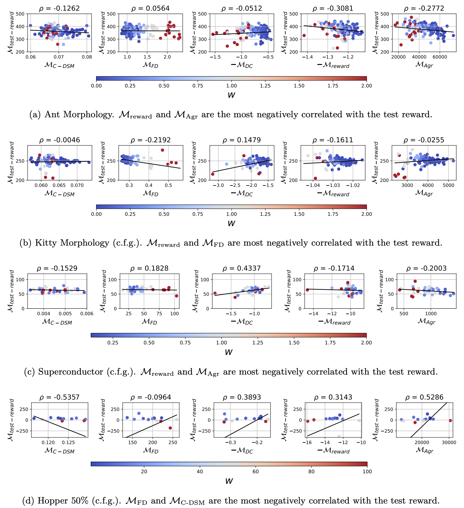
Some metrics are plotted as their negatives (e.g., \(-\mathcal{M}{\text{DC}}\) and \(-\mathcal{M}{\text{reward}}\)) to maintain consistency across all plots. Although these metrics are originally defined to be maximised, we negate them so that all metrics are presented as quantities to be minimised. Since this also applies to the test reward \(\mathcal{M}_{\text{test-reward}}\), the best validation metric is one which is the most strongly negatively correlated with it.
Since the above plots are a lot of information to process, we can just jump straight to the figure which barplots the Pearson correlation for each of these experiments:
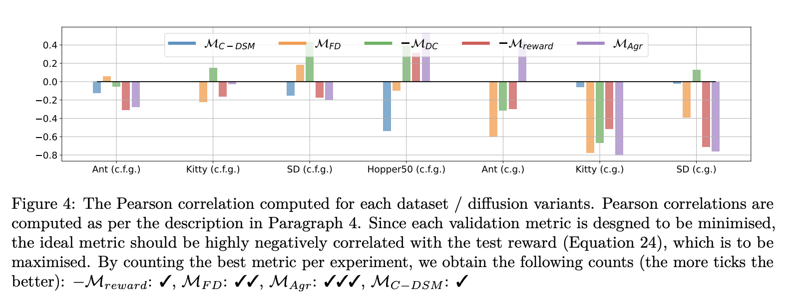
The above figure differs a little from the one before it, as we actually have three additional groups of experiments on the right corresponding to "c.g." in parentheses. These correspond to the "classifier guidance" variant of diffusion [11]. I won't go into details here, but you can think of this variant as really defining a special joint distribution \(\pt(x,y) \propto p_{\beta}(y|x)^{w}\pt(x)\) where \(p_{\beta}(y|x)\) is a regression model also trained on the training data. (So it's like a probabilistic form of "\(\ft\)", only that here we use subscript \(\beta\) as \(\theta\) is already assigned to the generative model.) Conversely, "c.f.g." [12] can simply be thought of as just \(\pt(x,y) = \pt(x|y)p(y)\) but with some algebra applied to Bayes' rule such that we condition on an "implicit" classifier \(\pt(y|x)\).
Overall, if we count which validation metric was most negatively correlated with the test reward for each dataset-guidance configuration, agreement is the most performant, followed by Frechet Distance.
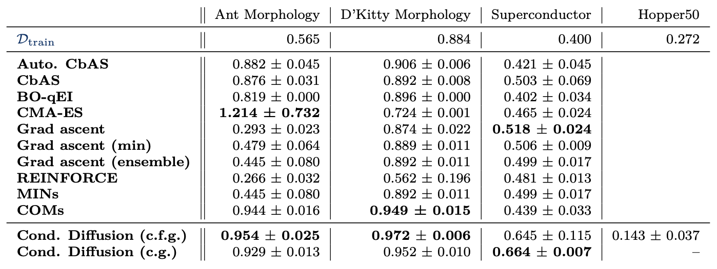
Lastly, the results we obtained are shown below in Fig. (7).
3. 🪵🔥 reflection, and future work
In the name of transparency and introspection, I will discuss what I think could have been done better.
The fundamental question we are trying to answer is: given a list of validation metrics a-priori, which are most useful as substitutes for the reward oracle? We exploited the fact that simulation environments exist – which grant access to the reward oracle – and then measure how correlated they are on four datasets. While this work isn’t about setting new benchmark records, the results are very encouraging (Fig. (7)). That said, it’s worth noting that this correlation is measured on the same data used to select the best metric, so there’s an inherent optimism bias. The ideal thing to do would have been to demonstrate that these metrics perform well on other downstream tasks. (The irony of this is not lost on me, but by the time I realised its significance I was very burned out from the project.)
The paper [1] was also tough to write, and honestly, so was this blog post. Maybe it’s because there were just too many ideas bouncing around at once: the importance of using a validation set, how to design that set to test extrapolation, thinking about MBO through the lens of generative modeling, and on top of that, proposing the use diffusion models – which, at the time, hadn’t really been explored in offline MBO. It would’ve been much simpler to just stick to the message of "validation sets, but for extrapolation". But at the time, that felt almost too obvious, like writing a paper just to say that validation sets are useful (which we already take for granted). But things that are supposedly "obvious" sometimes get published and go on to accrue hundreds of citations at the least, so maybe my barometer for that is miscalibrated.
I'm not sure how I would have approached the project if I did it again. When I reflect on past and ongoing industry work in similar problems, I notice a recurring pattern: we lean heavily on proxy metrics for validation. They’re cheap, measurable, and give us a sense of progress. But they’re also brittle and riddled with edge cases. It’s hard not to conclude that, sooner or later, all roads lead to human feedback models. It’s the only thing which consistently captures what we actually care about, even if it's noisy and expensive. So what does this mean then for this type of research? Maybe we ought to focus on best approximating the reward oracle and incorporate the best of both worlds in a single model: reliable, domain-specific priors, but also cheap and heterogenous sources of human feedback. The cost of obtaining labels is still an issue, but based on current trends it seems like the ever-increasing scale of foundation models will progressively allow for fewer-shot fine-tuning or prompting on top of them, which is a label efficient solution.
3.1. can we combine online and offline mbo?
Lastly, online and offline MBO feel somewhat siloed, when really one leads to another. Ideally, we want to build a good inductive prior in the offline setting and then segue into online to refine the model with real interactions. But in practice, offline MBO is only concerned with models which produce high-scoring samples "out of the box" with respect to the reward oracle, not whether that same model can be effectively used by an online learning algorithm to efficiently query it.
A real-world MBO workflow might appear as the following:
- (1) We start with offline data, e.g. past experiments, human preferences, etc.
- (2) Train a generative model on that data. It could be a conditional model \(\pt(x|y)\) or unconditional \(\pt(x)\). We may even decide to train a training proxy \(\ft(x)\) (which I will just "lump" into the generative model category).
- (3) Use generative model + some search algorithm to propose a small batch of high-scoring candidates and query those candidates with the reward oracle to obtain their labels.
- (4) Add the newly-obtained (input, label) pairs to the dataset.
- (5) Retrain or fine-tune the generative model on updated dataset.
- (6) Repeat steps (3)-(5) until budget is exhausted.
For (3), examples of "use generative model" may include:
- Using the generative model as a prior, e.g. if \(\pt(x,y)=\pt(x|y)p(y)\), then the search algorithm can initialise its starting point via a sample from \(\pt(x|y)\).
- The search algorithm uses either \(\pt(x)\) or \(\pt(x|y)\) to evaluate the density (i.e., the plausibility) of any input it has proposed. Evaluating the density is possible with certain models such as time-continuous diffusion [13] and normalising flows.
Here is a more concrete sketch of the algorithm with an added twist. First, to avoid any bias in assessing generalisation performance due to optimism, we use validation proxy \(\fvalid\) even during the online mode, and save the final evaluation with \(f\) until the very end. We also define a budget \(T_{\text{max}}\), which is how many evaluations we can perform in online mode:
- (1) Assume offline dataset \(\mathcal{D}\), split into \(\dtrain\), \(\dvalid\), and \(\dtest\). \(\fvalid\) is also trained on \(\dtrain \cup \dvalid\).
- (2) Train \(\pt\) on \(\dtrain\). (Here, \(\pt\) can refer to any density deemed useful, for instance \(\pt(x)\), or \(\pt(x,y)\).)
- (3) Online mode. For timestep \(t = 1, \dots, T\):
- (3a) Use \(\pt\) with search algorithm to sample a batch of high-scoring candidates.
- (3b) Obtain labels of candidates with \(\fvalid\), compute mean reward \(r_t\) over the batch, save this value.
- (3c) Update \(\tilde{\mathcal{D}}\) with previously obtained labels and fine-tune \(\pt\) with it.
- (4) Compute discounted sum of reward: \(G_T = \sum_{t=1}^{T} \gamma^{t-1}r_t\) for discount rate \(\gamma\).
The twist is an idea I took from RL, which is the discounted sum of rewards. This sum is meant to encode the notion that rewards obtained earlier carry larger weight than later, as each successive evaluation progressively increases the overall cost in querying the reward oracle. By choosing this as the validation metric, we favour generative models and search algorithms which produce high-scoring candidates as cheaply as possible.
(Hats off to my co-author Alex, who really instilled a sense of MBO needing to be cost-effective. I think this idea really hits at the heart of that.)
3.2. links, and open source
Here are some things you may find useful:
- 🛠️ [validation-metrics-offline-mbo]: the original code for my paper. This uses the DDPM style of diffusion model from Ho et al.
- 🛠️ [offline-mbo-edm]: this is a bit more minimalistic and has a more up-to-date diffusion model which is EDM. Not only is this more performant, it generalises existing diffusion models which grants a lot of flexibility when it comes to deciding how to sample.
Design Bench can take some time to setup, so whichever repo you look at I highly recommend you consult the installation readme I wrote here here. As of time of writing, the mainline branch for Design Bench has broken urls for its datasets, so you should switch to my branch:
git clone https://github.com/brandontrabucco/design-bench
git checkout chris/fixes-v2
cd design-bench
pip install . -e
4. References
Footnotes:
While online MBO also does a sort of hill climbing on the surrogate, the difference is that the resulting input is validated against the reward oracle, and this data is used to update the model.)
This should not be interpreted as discouraging "sim2real" experiments, where simulators are used to pre-train a model which is then adapted to a real world task. The difference is that if you treat the simulator as a training scaffold, then you need an external reward function to measure real performance. Otherwise, you're just evaluating on the same thing you are training on.
Conditional diffusion models are typically trained with dropout on the conditioning variable \(y\) (in our case, the reward). This makes them act as both unconditional and conditional models.
Continuous datasets were used as DDPM operates on continuous values. While discrete variants do exist, I did not explore these. The simplest way to extend this work to discrete datasets is to use a discrete VAE to encode samples into a continuous latent space and perform diffusion there instead.