EDM diffusion models - a Jupyter implementation, and how they are implemented in practice
1. Introduction
I wrote a self-contained implementation of NVIDIA's EDM in a Jupyter notebook. You may find it useful for the following reasons:
- You want to explore diffusion models on toy datasets (why? Because toy datasets train fast and require little compute);
- You want to understand diffusion models from a more fundamental perspective (toy datasets are great for that) (also see Ali Rahimi's NeurIPS '17 talk on why simple toy experiments are great);
- You want to try out new schedulers which fit under the particular framework proposed by EDM (e.g. defining novel parameterisations of \(\sigma(t)\) and \(s(t)\)).
- You want a "full" implementation of the general algorithms, i.e. being able to arbitrarily specify \(\sigma(t)\) and \(s(t)\). (The original repo hardcodes those parameterisations.)
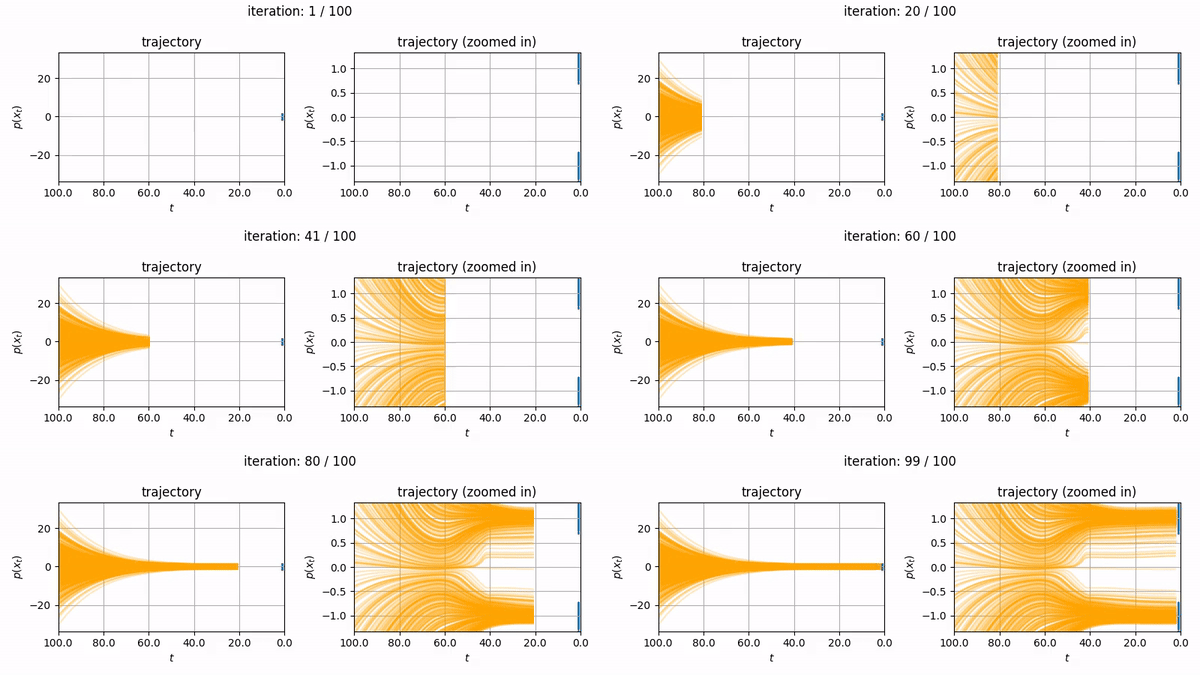
- You want to generate fun mp4's showing the diffusion trajectory of a 1D dataset (like below).
You can find the code here.

The notebook itself is self-contained and makes no reference to this blog post, however the following information may be useful to you if you want to know more about how EDM's algorithms are implemented for two major open source diffusion projects (diffusers and ComfyUI, the latter of which uses k-diffusion).
2. Schedulers
A particular class of scheduler algorithms implemented by k-diffusion (and by extension, ComfyUI and HuggingFace' diffusers) have rather opaque names because they don't clearly reflect their origins, nor are they complete implementations of the original algorithms from which they were derived. These algorithms are actually based on the "Algorithms 1 & 2" proposed in NVIDIA's EDM (Karras, Tero and Aittala, Miika and Aila, Timo and Laine, Samuli, 2022). Essentially, they are the deterministic and stochastic variants (respectively) of an ODE, one which was designed to encapsulate all of the different diffusion model variants used at the time. That ODE has the following form:
where: \(s(t)\) is some time-dependent scaling function of the input \(x\); \(\sigma(t)\) is the time dependent noise variable; and \(\dot{s}(t) = \frac{\partial s(t)}{\partial t}\) and \(\dot{\sigma}(t) = \frac{\partial \sigma(t)}{\partial t}\) . Along with other hyperparameters (such as how precisely the timesteps are discretised), this ODE is able to generalise the deterministic components of the sampling algorithms found in other papers.

Both algorithms are "somewhat" implemented in the following libraries:
k-diffusion, which takes the namesample_heun.diffusers, which takes the nameHeunDiscreteScheduler;- Both have more computationally efficient variants (i.e. without the second order steps) called
sample_eulerandEulerDiscreteScheduler, respectively; - but there are differences to the original paper and sometimes the implementations are not complete (in the case of
diffusers).
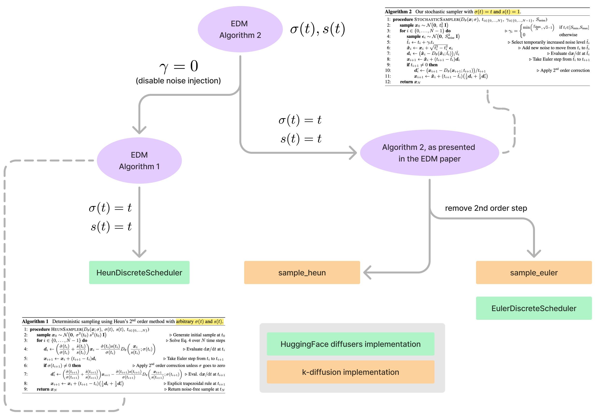
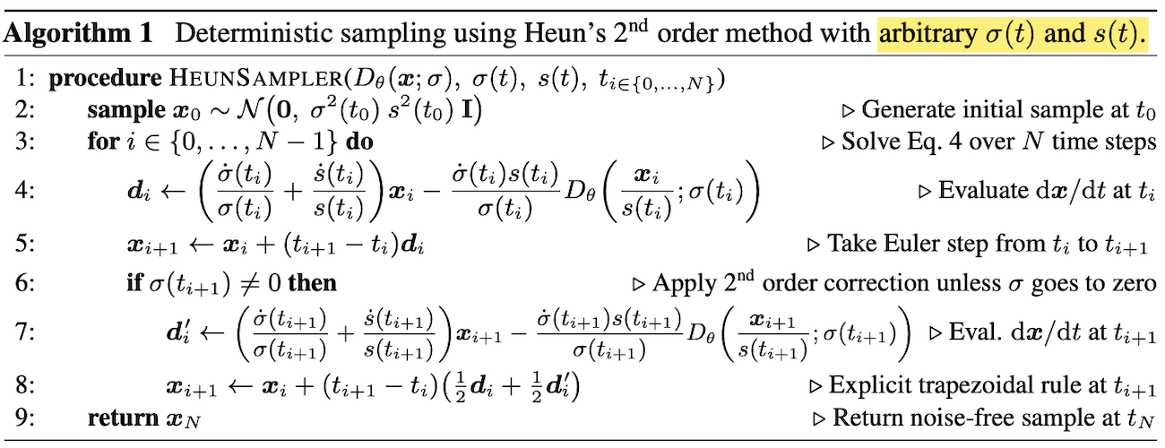
The way Algorithm 1 is presented in the EDM paper (Karras, Tero and Aittala, Miika and Aila, Timo and Laine, Samuli, 2022) is "general" since it assumes no particular \(\sigma(t)\) and \(s(t)\) (see Figure 2). In terms of how they are implemented in practice:
- In k-diffusion it's called
sample_heun, but only if we pass \(\gamma = 0\) into the function so that the stochastic part (the noise injection component proposed by Alg. 2) disappears. Also it's assumed \(\sigma(t)=t\) and \(s(t)=1\), so it's not the general form of the algorithm as shown in Fig. 2. - In diffusers it's called
HeunDiscreteScheduler. Also it's the same parameterisation as k-diffusion, but \(\gamma = 0\) is only supported (as of 21/06/2024) which means that it literally does turn into Algorithm 1. (The reason for only supporting \(\gamma = 0\) seems to stem from the awkwardness of the fact that the the U-Net backbones indiffusersrequire discrete indices to be passed to the forward method instead of continuous values, which means one would have to back-calculate the appropriate "timestep" from \(\hat{\sigma}\).)
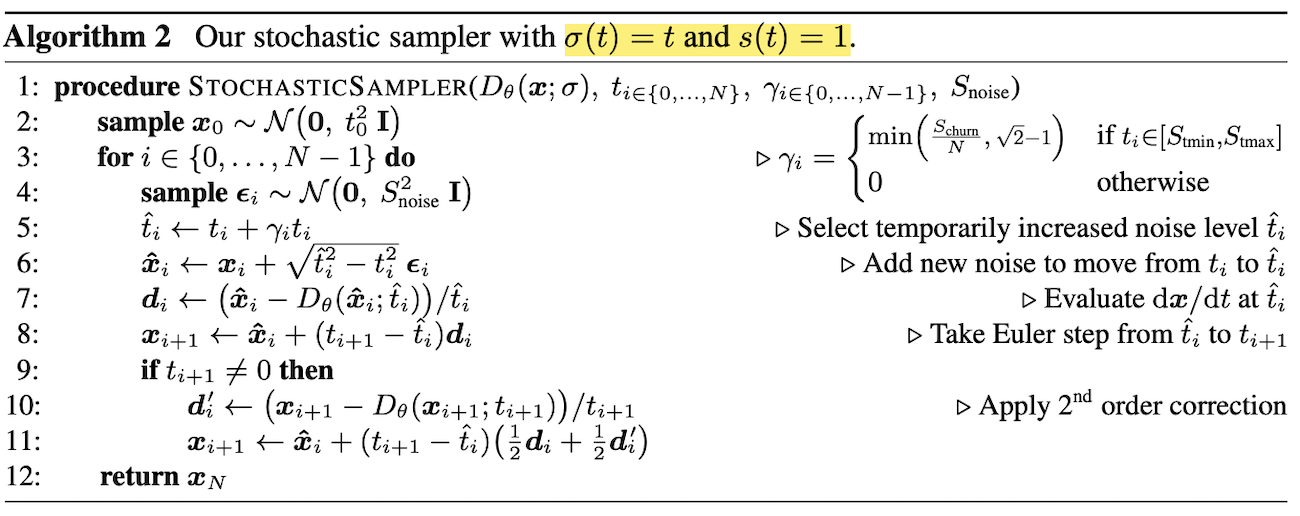
Algorithm 2 in (Karras, Tero and Aittala, Miika and Aila, Timo and Laine, Samuli, 2022) is basically a stochastic variant of Algorithm 1, but the paper does not present the general form of the algorithm. Rather, it assumes \(\sigma(t) = t\) and \(s(t) = 1\) (see Figure 2). In terms of code:
- k-diffusion implements it with that specific choice of \(\sigma(t)=t\) and \(s(t)=t\).
- For
diffusers,HeunDiscreteSchedulerdoes not support \(\gamma > 0\) yet and so there is no support for Algorithm 2 per se. However,EulerDiscreteSchedulerdoes (confusingly). - While the specific choices of \(\sigma(t)\) and \(s(t)\) are well justified (they perform the best empirically), having the more general forms of the algorithms would open them up to exploring different forms of the general ODE.
Quite frankly, I'm not the biggest fan of these scheduler names because they don't reflect the fact they are EDM-specific algorithms (even if the attribution is there in the docstrings). Why can't we simply just implement one mega-algorithm called edm_sampler and allow the option for a use_second_order flag as well as gamma so that it encapsulates everything? Or at least use class names like edm_deterministic_sampler, edm_stochastic_sampler, etc. I suppose the reason whh they are named so "generically" (for lack of a better term) is that the general-form ODE proposed by EDM really does encompass (as of time of writing) "more or less" all of the diffusion variants commonly used. Therefore, to just give it a name like "{Euler,Heun}DiscreteScheduker" is not unreasonable.
Lastly, there is one additional algorithm which shares the same naming convention as the others but really has nothing to do with the EDM paper. This is the "ancestral sampling algorithm" based off Jonathon Ho's DDPM paper (Ho, Jonathan and Jain, Ajay and Abbeel, Pieter, 2020). In diffusers it's called EulerAncestralDiscreteSampler (see here) and in k-diffusers it's called sample_euler_ancestral (see here). More info on that is in Sec. 2.1.


2.1. Ancestral sampler
Both k-diffusion and diffusers have a version of the Euler-based version of Algorithm 2. To make matters even more confusing, the sample_euler_ancestral algorithm is basically the Euler variant of Algorithm 2 but with the EDM-specific noise injection mechanism cut out in favour of ancestral sampling. Ancestral sampling is detailed in Appendix F of the continuous-time score matching paper from Song et al. (Song, Yang and Sohl-Dickstein, Jascha and Kingma, Diederik P and Kumar, Abhishek and Ermon, Stefano and Poole, Ben, 2020). The update rule for this is:
where \(s_{\theta}(x, \sigma) = (x - D(x; \sigma) / \sigma^2\) and \(z_i \sim \mathcal{N}(0, \mathbf{I})\). (Unlike in (Song, Yang and Sohl-Dickstein, Jascha and Kingma, Diederik P and Kumar, Abhishek and Ermon, Stefano and Poole, Ben, 2020), I am being consistent with the rest of this post by denoting \(\sigma_0\) as the highest noise scale as \(\sigma_{T-1}\) as the smallest.)
This equation can basically be seen as doing the ODE step (the first two terms on the RHS) but then injecting noise \(\sim \mathcal{N}(0, \sigmaup)\). For reasons not clear to me yet, this is not the exact same as what's implemented in k-diffusion (see here and here), which implements something seemingly a lot more complicated:
\begin{align} x_{i+1} = x_i + (\sigmadown - \sigma_{i}) s_{\theta}(x_i, \sigma_i) + \underbrace{\text{min}\Big(\frac{\sigma_{i+1}}{\sigma_i} \sqrt{\sigma_i^2 - \sigma_{i+1}^2}, \sigma_{i+1}\Big)}_{\sigmaup} z_i, \end{align}and \(\sigmadown = \sqrt{\sigma_{i+1}^2 - \sigmaup^2}\). (I've also redefined \(\sigmaup\) here to also include the min.) (If anyone knows more about this, please reach out so I can update this post.)
3. Conclusion
In conclusion, I have shared a Jupyter implementation of EDM on toy datasets, as well as elucidate (pun intended) some of the opaque naming conventions used in the practical implementations which implement EDM's algorithms.