A deep dive into conditional variational autoencoders
Updates:
- (06/10/2023) Some fixes to the text, and an overhaul of the discussion section to connect it better with the rest of the post.
Table of Contents
1. Introduction
This is yet another excerpt from my upcoming PhD thesis. I actually wanted to write this several years ago after some really painful experiences I had with getting conditional VAEs to work on a generative modelling project I was working on. To the best of my knowledge, I haven't seen any paper that talks in depth about these difficulties and so I am quite happy to finally share them with everyone. VAEs – despite their conceptual simplicity – can be difficult to understand and even more so for its conditional variants. In this post I will dive into the theory of conditional VAEs, derive interesting equations which elucidate their behaviour, and corroborate those insights on a simple toy dataset.
1.1. Contributions
This post focuses almost exclusively on conditional VAEs, but it also equally applies to unconditional ones. The contributions of this post are as follows:
- In Section 2 we present cVAEs through an unconventional but rather enlightening perspective, inspired by Esmaeili et al. (2018). This involves thinking about the VAE as parameterising two separate pathways (the generative and inference process), and the evidence lower bound can be derived as the KL divergence between these two. While their work was derived assuming unconditional VAEs, we consider the conditional case as well.
- We discuss two parameterisations of a cVAE: one where the conditioning variable \(\yy\) and latent variable \(\zz\) are assumed to be either independent (Section 2.1) or dependent (Section 2.2). The former is a useful parameterisation if one is interested in performing controllable generation.
- Through the lens of mutual information estimation, we elucidate the difficulties involved in training such a class of models (Section 2.4). In particular, we show such that optimising VAEs is a careful balance between ensuring that sample quality and diversity are adequate for both the generative and inference processes.
- We present experiments corroborating our theoretical analyses on a toy 2D dataset consisting of two Gaussian clusters, where a cVAE must be trained to sample from either of the two clusters correctly (Section 3).
- We discuss how VAE training issues can be avoided by considering adversarial learning or hybrid adversarial / VAE-style models.
2. The generative and inference process
VAEs are typically derived by starting off by assuming a latent variable model of the form \(\pt(\xx,\zz)\), and noting that integrating this expression over \(\zz\) to obtain \(\pt(\xx)\) is intractable. There is a further assumption that \(\pt(\xx,\zz) = \pt(\xx|\zz)p(\zz)\), but we also don't know what inputs \(\xx\) correspond to what \(\zz\), and since deriving \(\pt(\zz|\xx)\) is also intractable we need to introduce a separate network \(\qp(\zz|\xx)\) to do the job for us.
Inspired by esmaeili2018structured, we can actually derive the ELBO for a VAE by framing the training objective as a minimisation over the KL divergence between two pathways, each encoded by their own joint distribution. (We already saw the first of these joint distributions previously, which is the generative distribution denoted \(\pt\).) Since we're also talking about conditional VAEs, we will be dealing with an additional latent variable \(\yy\), but unlike \(\zz\) we have labels for this. We assume that \(\yy\) encodes some semantic meaningful label of interest, for instance the class of a digit, or the identity of an object.
The first pathway is the inference process, denoted \(\qp(\xx,\zz,\yy)\). It factorises into \(\qp(\zz|\xx,\yy)q(\xx,\yy)\), and to obtain a sample \((\zz,\xx,\yy)\) from this joint we simply perform the following:
\begin{align} \label{eq:inference} \xx, \yy & \sim q(\xx, \yy) \ \ \text{(ground truth)} \tag{2a} \\ \zz & \sim \qp(\zz|\xx, \yy) \tag{2b} \end{align}where \(q(\xx,\yy)\) is the ground truth data distribution, and \(\qzgivenx\) is our learnable variational posterior, subscripted with \(\phi\). The inference process is concerned with extracting latent representations from actual samples from the data distribution. This is to be contrasted with the generative process, in which samples are generated as the following:
\begin{align} \label{eq:generative} \zz, \yy & \sim p(\zz,\yy) \tag{3a} \ \ \text{(prior)} \\ \xx &\sim \pt(\xx|\zz,\yy) \tag{3b}, \end{align}where \(p(\zz,\yy)\) is prescribed beforehand. (We will talk a little more about this shortly.)
Since joint distribution for both processes are \(\ptgreen(\xx,\zz,\yy)\) and \(\qp(\xx,\zz,\yy)\) and we can derive their KL distribution as follows:
\begin{align} \label{eq:case1} \argmax_{\color{green}{\theta}, \color{purple}{\phi}} & -\kldiv \Big[ \qp(\XX,\ZZ,\YY) \ \| \ \ptgreen(\XX,\ZZ,\YY) \Big] \\ & = \mathbb{E}_{\qp(\xx,\zz,\yy)}\big[ \log \frac{\pt(\xx,\zz,\yy)}{\qp(\xx,\zz,\yy)} \big] \tag{4a} \\ & = \mathbb{E}_{\qp(\zz|\xx,\yy)}\big[ \log \frac{\pt(\xx | \yy, \zz)p(\yy,\zz)}{\qp(\zz|\xx,\yy)} \big] - \mathbb{E}_{q(\xx,\yy)} \log q(\xx, \yy) \tag{4b} \\ & = \mathbb{E}_{\qp(\xx,\zz,\yy)}\big[ \log \frac{\pt(\xx | \yy, \zz)p(\yy, \zz)}{\qp(\zz|\xx,\yy)} \big] - \text{const.} \tag{4c} \\ & = \mathbb{E}_{\qp(\xx,\zz,\yy)} \big[ \log \pt(\xx|\yy,\zz) \big] + \mathbb{E}_{\qp(\zz|\xx,\yy)} \big[ \log \frac{p(\yy, \zz)}{\qp(\zz|\xx,\yy)} \big] - \text{const.} \tag{4d} \\ & = \mathbb{E}_{\qp(\zz,\xx,\yy)}\big[ \log \pt(\xx|\yy,\zz) \big] - \kldiv\Big[ \qp(\ZZ|\XX, \YY) \| p(\ZZ,\YY)\Big], \tag{4e} \end{align}which gives us the typical formulation of the ELBO which we see in most VAE papers.
2.1. When z and y are independent
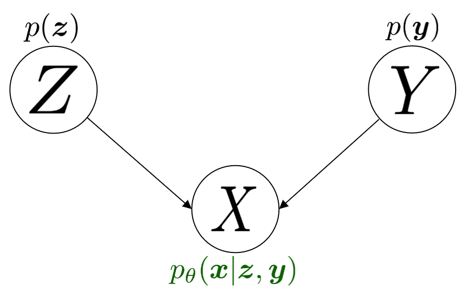
At this point, we have to specify what \(p(\zz,\yy)\) is, and we have two options. The first is to assume that \(p(\zz,\yy) = p(\zz)p(\yy)\), i.e. they are independent. This means that the joint distribution of the generative process factorises into:
\begin{align} \pt(\xx,\zz,\yy) = \pt(\xx|\zz,\yy)p(\zz)p(\yy) \tag{5} \end{align}which leads us to the following ELBO:
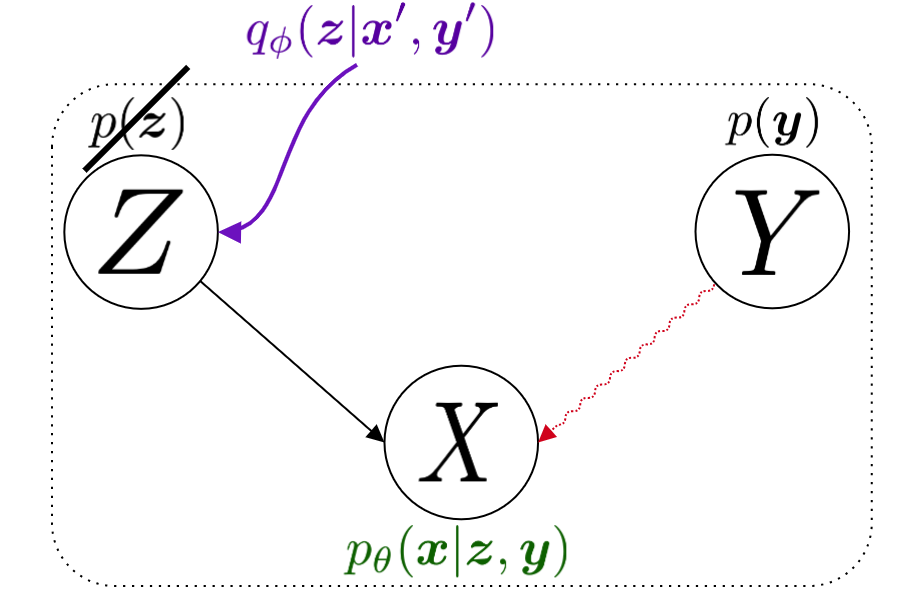
\begin{align} & -\kldiv \Big[ \qp(\XX,\ZZ,\YY) \ \| \ \ptgreen(\XX,\ZZ,\YY) \Big] \tag{6a} \\ & \myeq{\text{if ind.}} \mathbb{E}_{\qp(\zz,\xx,\yy)}\big[ \log \pt(\xx|\yy,\zz) \big] + \mathbb{E}_{\qp(\zz,\xx,\yy)}\big[ \log \frac{\pgreen(\zz)}{\qp(\zz|\xx,\yy)} \big] + \log \pgreen(\yy) \tag{6b} \\ & = \text{likelihood} - \kldiv\Big[ \qp(\ZZ|\XX,\YY) \| p(\ZZ) \Big] + \text{constants}. \tag{6c} \end{align}Here, \(p(\yy)\) is some prior for \(\yy\) but it falls out of the KL term since it is a constant, so we need not worry about it. All that is left is to define a prior for \(p(\zz)\), and in practice this is most often an isotropic Gaussian distribution. The graphical model for the \(\color{green}{\text{generative process}}\) is also shown in Figure 1.
Such a factorisation may be useful to encode if we are seeking to learn disentangled representations. For instance, if we were learning a conditional VAE over SVHN digits (where \(y\) encodes the identity of the digit), perhaps we would like for our VAE to learn a \(\zz\) that encodes \emph{everything else} in the image apart from the digit itself (for instance background details and font style). This would make for a very controllable generative process where we could arbitrarily mix and match style and content variables from different examples to create new ones.
2.2. When z and y are dependent
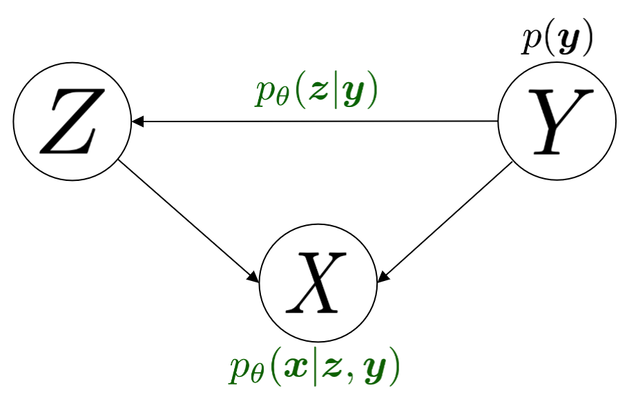
Otherwise, \(\pgreen(\zz,\yy) = \pgreen(\zz|\yy)\pgreen(\yy)\) and \(\pgreen(\zz|\yy)\) is the conditional prior. This means that the joint distribution factorises into:
\begin{align} \pt(\xx,\zz,\yy) = \pt(\xx|\zz,\yy)p(\zz|\yy)p(\yy) \tag{7} \end{align}The conditional prior can either be fixed (i.e. each possible value of \(\yy\) gets mapped to a Gaussian), or it can be learned, in which case we denote it as \(\pt(\zz|\yy)\). In this case the ELBO can be written as:
\begin{align} & -\kldiv \Big[ \qp(\XX,\ZZ,\YY) \ \| \ \ptgreen(\XX,\ZZ,\YY) \Big] \tag{8a} \\ & = \mathbb{E}_{\qp(\zz,\xx,\yy)}\big[ \log \pt(\xx|\yy,\zz) \big] + \mathbb{E}_{\qp(\zz,\xx,\yy)}\big[ \log \frac{p(\zz|\yy)}{\qp(\zz|\xx,\yy)} \big] + \log p(\yy) \tag{8b} \\ & = \text{likelihood} - \kldiv\Big[ \qp(\ZZ|\XX,\YY) \ \| \ p(\ZZ|\YY) \Big] + \text{constants}. \tag{8c} \end{align}Consequently, the graphical model for the \(\color{green}{\text{generative process}}\) is shown in Figure 2.
2.3. The role of the beta term
Let us look at both versions of the ELBO, equations 6(c) and 8(c), and write them as minimisations over \(\thetagr, \phip\):
\begin{align} \text{dep.} \rightarrow & \min_{\thetagr, \phip} -\mathbb{E}_{\qp(\zz,\xx,\yy)}\big[ \log \pt(\xx|\yy,\zz) \big] + \beta\kldiv\Big[ \qp(\ZZ|\XX,\YY) \ \| \ p(\ZZ|\YY) \Big] \tag{9a} \\ \text{indep.} \rightarrow & \min_{\thetagr, \phip} -\mathbb{E}_{\qp(\zz,\xx,\yy)}\big[ \log \pt(\xx|\yy,\zz) \big] + \beta\kldiv\Big[ \qp(\ZZ|\XX,\YY) \ \| \ p(\ZZ) \Big] \tag{9b}, \end{align}where 'dep' and 'indep' are shorthand for 'dependent' and 'independent'. Also note that since the independent case is assuming \(p(\zz,\yy) = p(\zz)p(\yy)\) we could also define \(\qp(\zz|\xx,\yy) = \qp(\zz|\xx)\) to remove the dependence on \(\yy\), but to keep notation consistent we will leave it in for the remainder of this post.
What makes VAE training difficult to get right is the interplay between the two terms in each equation. The first equation is maximising the likelihood of the data with respect to samples from the inference network. In order for this to happen, \(\zz\) should encode as much information about \(\xx\) as possible through the variational posterior \(\qp\), which is our learned encoder. At the same time however, the second term is working against the first, because it is enforcing that each per example variational posterior must be close to the prior distribution1. Since the prior is not a function of \(\XX\) it implies that some information about \(\XX\) in the encoding pathway has to be lost. Essentially, we are trading off between sample quality with respect to:
- the inference pathway, which is \(\qp(\zz,\xx,\yy) = \qp(\zz|\xx,\yy)q(\xx,\yy)\), where \(q(\xx,\yy)\) is the ground truth joint distribution;
- and the generative pathway, which is \(\pt(\zz,\xx,\yy) = p(\zz,\yy)\pt(\xx|\zz,\yy)\),
and hence why it is useful to know that the evidence lower bound in Eqn. (9) is a direct result of minimising the KL divergence between those two distributions.
In practice, what one observes with a VAE as a function of \(\beta\) is the following:
- if \(\beta\) is too small then samples from the prior distribution \(\zz \sim p(\zz)\) will not look as good as samples from the variational encoder \(\zz \sim \qp(\zz|\xx,\yy)\);
- if \(\beta\) is too large then sample quality with respect to both will be degraded, and hence the search for \(\beta\) is a careful balance between the two extremes;
- and if \(\beta\) is 'just right', sample quality with respect to both should be 'ok'.
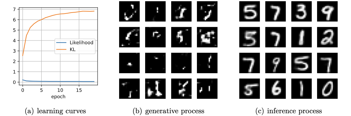
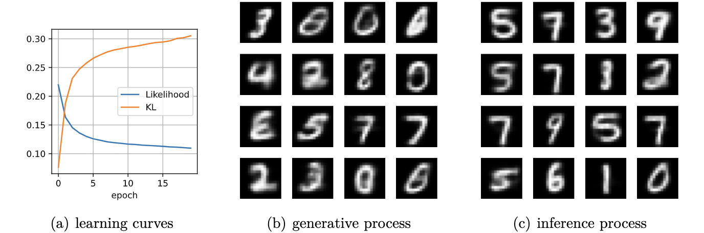
In Figure 5 we show images from an unconditional VAE illustrating this trade-off for MNIST.
2.4. A mutual information perspective for the KL term
This aforementioned loss of information due to \(\kldiv\big[ \qp(\ZZ|\XX,\YY) \ \| \ p(\ZZ, \YY) \big]\) can be theoretically shown, by re-writing the KL term to be the sum of a mutual information term and another KL divergence term.
For the dependent case:
\begin{align} \text{dep.} & \rightarrow \kldiv \Big[ \qp(\ZZ|\XX,\YY) \| p(\ZZ|\YY) \Big] \\ & = \mathbb{E}_{\qp(\zz,\xx,\yy)} \log \frac{\qp(\zz|\xx,\yy)}{p(\zz|\yy)} \tag{10a} \\ & = \mathbb{E}_{\qp(\zz,\xx,\yy)} \log \Big[ \frac{\qp(\zz|\xx,\yy)}{p(\zz,\yy)} \cdot \frac{\qp(\zz)}{\qp(\zz)} \Big] \tag{10b} \\ & = \mathbb{E}_{\qp(\zz,\xx,\yy)} \log \Big[ \frac{\qp(\zz|\xx,\yy)}{\qp(\zz)} \cdot \frac{\qp(\zz)}{p(\zz,\yy)} \Big] \tag{10c} \\ & = \mathbb{E}_{\qp(\zz,\xx,\yy)} \log \frac{\qp(\zz|\xx,\yy)}{\qp(\zz)} + \mathbb{E}_{\qp(\zz,\yy)} \frac{\qp(\zz)}{p(\zz,\yy)} \tag{10d} \\ & = I_{\phip}(\ZZ; \XX, \YY) + \kldiv[ \qp(\ZZ) \| p(\ZZ|\YY) ] - \underbrace{\mathbb{E}_{\qp(\yy)} \log p(\yy)}_{\text{const}} \tag{10e} \end{align}Similarly, for the independent case we obtain:
\begin{align} \text{indep.} & \rightarrow \kldiv \Big[ \qp(\ZZ|\XX,\YY) \| p(\ZZ) \Big] \nonumber \\ & = \kldiv \Big[ \qp(\ZZ|\XX) \| p(\ZZ) \Big] \nonumber \\ & = I_{\phip}(\ZZ; \XX, \YY) + \kldiv[ \qp(\ZZ) \| p(\ZZ) ] - \text{const}. \tag{10f} \end{align}In either of the two cases, the minimisation of their respective KL terms implies minimising the mutual information between \(\XX\) and the pair \((\ZZ,\YY)\), denoted as \(I_{\phip}(\ZZ; \XX, \YY)\). Therefore, when we increase \(\beta\) we are inevitably reducing the information \(\ZZ\) stores about \(\XX\) with respect to the encoder \(\qp\).
2.5. A mutual information perspective between Z and Y
In the previous section we showed how minimising the KL term in the ELBO involves also minimising the mutual information between \(\ZZ\) and \(\XX,\YY\) through its decomposition in Eqn. (10e) and (10f), and that it is a consequence of trying to match the generative and inference distributions. Furthermore, the extent to which we try to minimise this equation affects the relative difference in sample quality between \(\zz\)'s which are sampled from the prior distribution versus ones generated with the variational distribution.
Minimising the mutual information between \(\ZZ\) and \(\YY\) for \(\ZZ,\YY\) independent VAEs is also important since we want the two variables to encode completely separate concepts. For instance, it is common in image datasets for \(\YY\) to encode something semantically desirable about \(\XX\), for instance the identity of the object in the foreground or what category it belongs to. If our dataset is labelled such that \(\YY\) is assigned such semantic meaning, then we would like \(\ZZ\) to encode everything else that is not related to \(\YY\).
From Sec. 2.4 we showed that minimising the per-example KL means also minimising \(I_{\phip}(\XX; \ZZ)\). In actuality it would be nice to instead minimise the mutual information between \(\ZZ\) and \(\YY\) (even though this term is not present in the equation), but the issue is that \(\XX\) \emph{also encodes} information about \(\YY\), and so trying to drive down \(I_{\phip}(\ZZ; \YY)\) would inevitably mean we need to drive down \(I_{\phip}(\ZZ; \XX)\), but this degrades sample quality2. In the absence of extra supervisory signal3 that could potentially encourage the network to only encode the `non-label' parts of \(\XX\) in \(\ZZ\), we are stuck with a very difficult optimisation problem.
2.5.1. Practical considerations
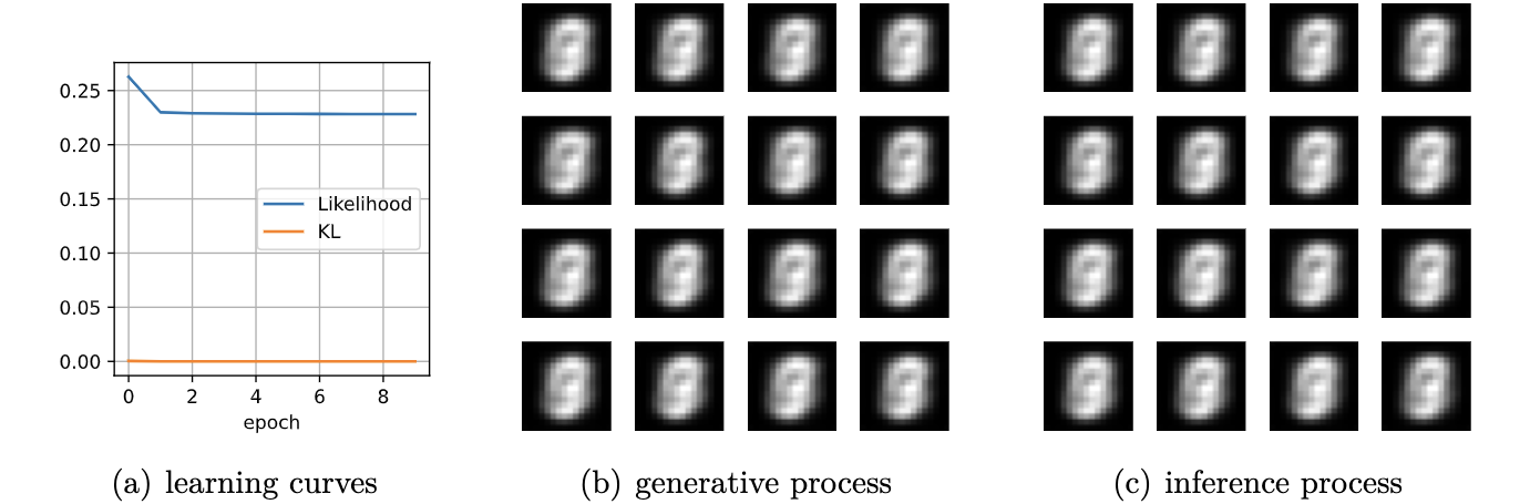
In practice, if the KL term is not large enough (Eqn. (9b)) then the decoder \(\pt(\xx|\zz,\yy)\) will ignore the \(\YY\) variable. This is presumably because \(\ZZ\) will contain too much information about \(\YY\) which in turn renders it irrelevant with respect to the decoder (Figure 6). This is an issue because it prevents us from performing controllable generation. Essentially, given some input \(\xx\) if we can encode it into its (independent) factors of variation \(\zz, \yy\) then we could easily swap out \(\yy\) with a new label \(\yy'\) and decode to produce a different kind of output (see Sec. 6.4 for an example):
\begin{align} (\xx, \yy) & \sim \mathcal{D} \tag{12a} \\ \yy' & \sim p(\yy) \tag{12b} \\ \zz & \sim \qp(\zz|\xx,\yy) \tag{12c} \\ \xx' & \sim \pt(\xx|\zz,\yy') \tag{12d} \end{align}If the KL term is not weighted high enough however then \(\yy'\) won't make any difference whatsoever. Unfortunately, it is difficult to tell whether this is happening through monitoring the ELBO. Basically, one will need to figure out via cross-examination what the 'largest' value for the KL term can be before \(\yy\) gets ignored by the decoder.
3. Experiments
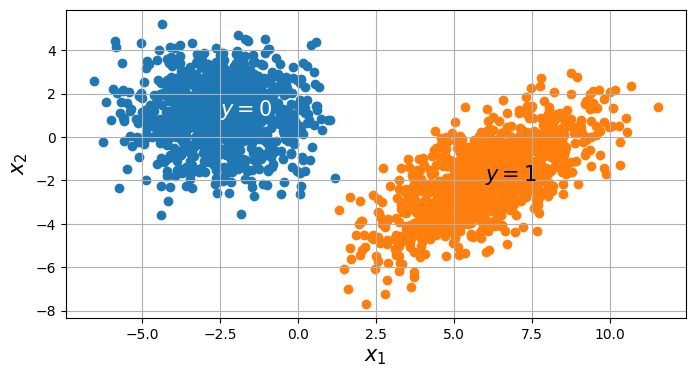
We now present some experiments on a toy 2D dataset for both variants of cVAE. The dataset consists of two Gaussians, and the ground truth is:
\begin{align} p(\xx) = \sum_{i \in \{0,1\} }p(\xx,\yy_i) = \sum_{i \in \{0,1\}} p(\xx|\yy_i)p(\yy_i), \end{align}where \(p(\xx|\yy=0) = \mathcal{N}(\xx; [-2.5, 1]^{T}, 2\mathbf{I})\), \(p(\xx|\yy=1) = \mathcal{N}(\xx; [6,-2]^{T}, 2 + \mathbf{I})\), and \(p(\yy=0) = p(\yy=1) = \frac{1}{2}\). Samples from this distribution are visualised below in Figure 3.
For the following experiments, we train a single hidden layer MLP for both the encoder and decoder. The encoder is a mapping \(\mathbb{R}^{2} \rightarrow \mathbb{R}^{h} \rightarrow \mathbb{R}^{2}\) which means the latent variable is also two-dimensional, for interpretability sake. Likewise, the decoder is of a similar mapping.
For the following experiments, we wish to illustrate the behaviour of a conditional VAE with respect to the following attributes: (1) whether \(\ZZ\) and \(\YY\) are dependent or not; (2) as a function of increasing the KL regularisation coefficient \(\beta\). Furthermore, we wish to illustrate both behaviours in input space \(\mathcal{X}\) as well as latent space \(\mathcal{Z}\). For convenience, both the input and latent spaces are two-dimensional, and subsequent figures will make it clear which space is being visualised.
Concretely, the encoder \(\qp(\zz|\xx)\) is an MLP \(\mathbb{R}^{p=2} \rightarrow \mathbb{R}^{h} \rightarrow \mathbb{R}^{p=2}\) for \(h\) hidden units. Likewise, the decoder takes on a similar structure.
3.1. When z and y are independent
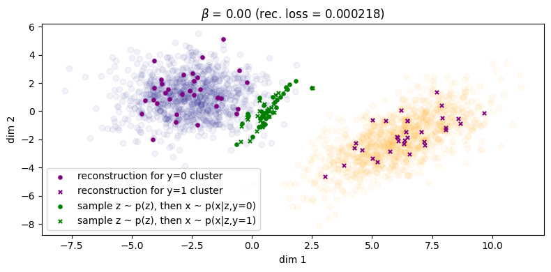
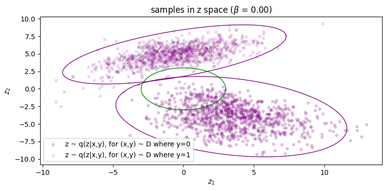
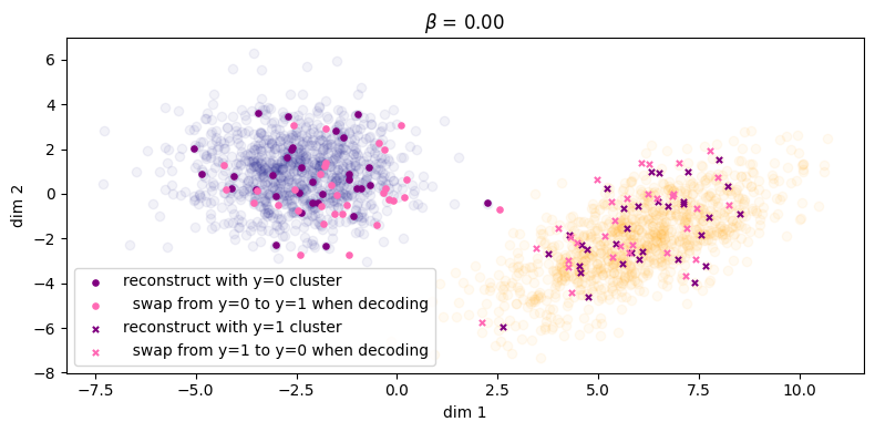
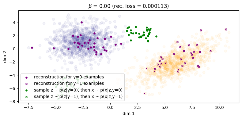
First we show \(\beta = 0\), illustrated in Figure 3. Samples from the inference process are shown in \(\color{purple}{\text{purple}}\) and those from the generation process in \(\color{green}{\text{green}}\), similar to the notation that we have been using so far in the equations. For instance if we consider the inference process: for a given \((\xx, \yy)\) from the data distribution, we sample \(\zz \sim \qp(\zz|\xx,\yy)\) and then we reconstruct by sampling \(\tilde{\xx} \sim \pt(\xx|\zz,\yy)\). The corresponding reconstruction error is shown in the title (the squared L2 norm between the original points and their reconstructions), and we can see that the error is small enough we can essentially consider it to be zero. However, things don't look so good for the generative process: for a given \(\zz \sim p(\zz)\), we can either choose to decode with \(\pt(\xx|\zz,\yy=0)\) or \(\pt(\xx|\zz,\yy=1)\), and these more or less fall in the same region. This indicates that choosing \(\yy\) does not make a difference to the generated samples (recall Fig. 6 in Sec. 2.5.1). What we would like to see is the samples from the prior falling into their respective clusters.
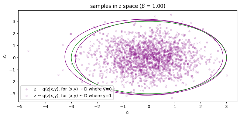
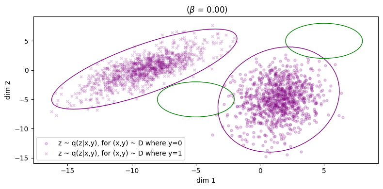
We can also visualise samples in latent space as well as the distributions for \(p(\zz)\) as well as the conditional inference distributions \(\qp(\zz|\yy_i)\), and this is shown below in Fig. (3b). (Note that \(\qp(\zz)\) the inference marginal itself is also just the weighted sum of both of these distributions, weighted by their prior probability \(q(y=i)\).)
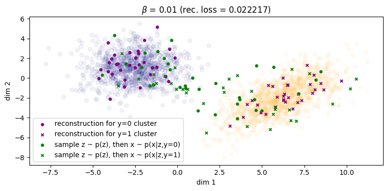
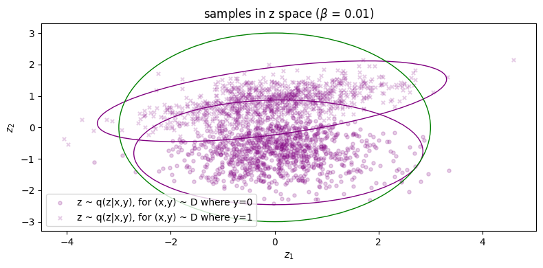
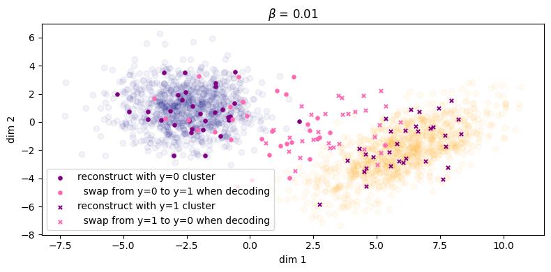
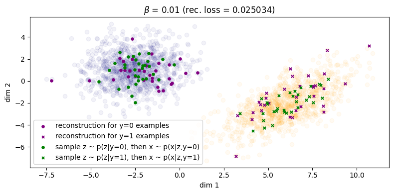
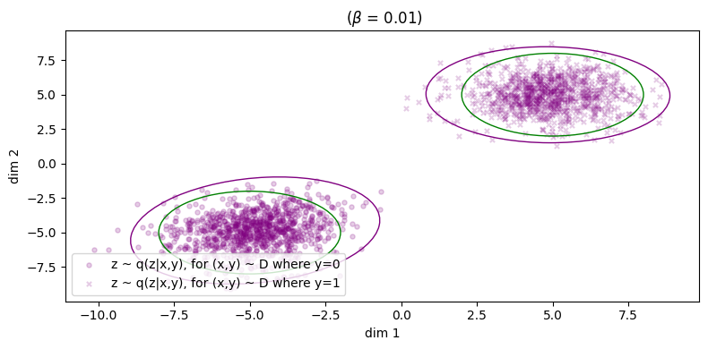
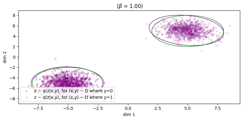
In Figure 4a, if we choose \(\beta = 0.01\), it looks as though some of the green points have been pulled to their respective cluster but there is still some overlap between the two categories and we don't see any clear pattern of separation. At the very least, sample diversity is superior to that in Figure 1 because at least the green points are sufficiently spread out to cover the two clusters of the data. The reconstruction error for the inference process has only taken a minor hit, increasing from roughly zero to \(\approx 0.02\). In Figure 4b, we can see that the marginal \(\qp(\zz)\) is a little closer to the prior, but it's still easy to make out the two separate clusters belonging to the different \(\yy\)'s, so \(I_{\phip}(\ZZ; \XX, \YY)\) is still reasonably large.
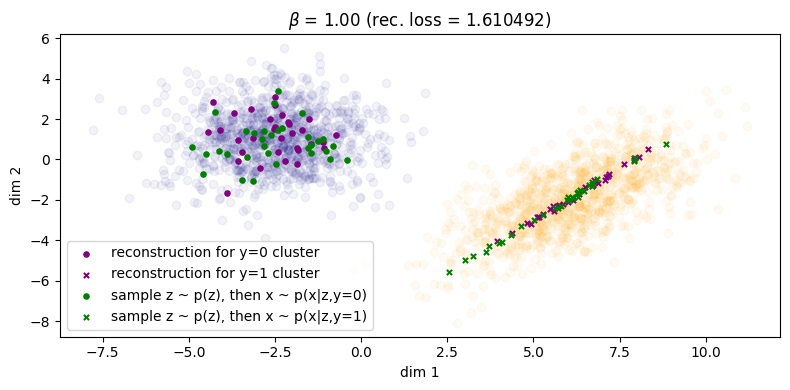
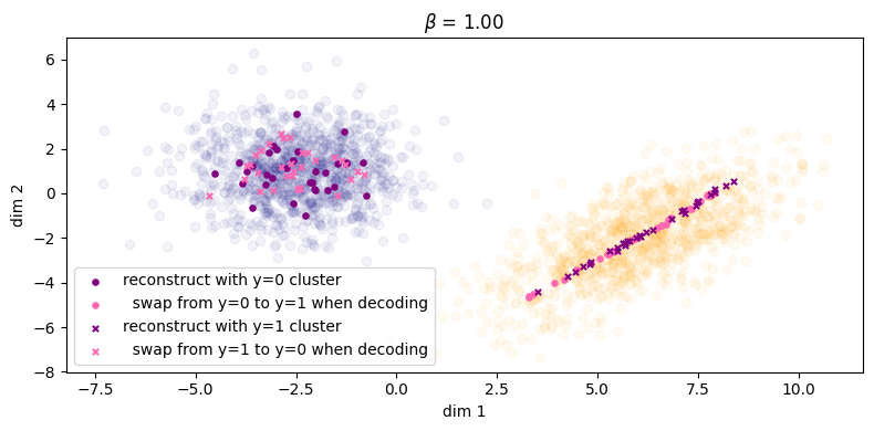
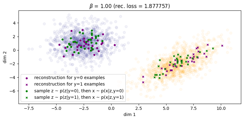
Finally, in Figure 5 for \(\beta = 1\) we finally see that the green points get matched to their respective clusters. Unfortunately, the inference process has degraded and reconstruction error has significantly increased as as result (\(\approx 1.61\)). We can also see this qualitatively for the rightmost cluster, where reconstructions lie on a very narrow subspace instead of being more evenly distributed across the cluster. Therefore, we can say that with respect to both processes, sample quality is \emph{very good} but sample diversity has \emph{degraded}. Lastly, note that in Figure 5b the two condtionals \(\qp(\zz|\yy=0)\) and \(\qp(\zz|\yy=1)\) are more or less the same, which indicates roughly zero mutual information between \(\ZZ\) and \(\YY\). Because of this, the autoencoder will now be `incentivised' to make use of \(\yy\) since it will obviously be a useful variable to leverage use when maximising the log likelihood of the data (assuming \(\beta\) is not too large, since it controls the degree to which the optimisation focuses on the likelihood term).
3.1.1. Controllable generation
One benefit of training a \(\ZZ,\YY\) independent VAE is that we can perform controllable generation more easily (or at least hope to) compared to the dependent variant. For instance, if \(\ZZ\) and \(\YY\) encode the non-semantic and semantic parts of the input, we could generate a novel example by combining the semantic content of one input with the non-semantic content of another. In this case, \(\YY\) is a binary random variable indicating the cluster:
\begin{align} (\xx,\yy) & \sim \mathcal{D} \tag{13a} \\ \zz & \sim \qp(\zz|\xx,\yy) \tag{13b} \\ \xx' & \sim \pt(\xx|\zz,1-\yy) \tag{13c} \end{align}Similar to Sec. 3.1 we illustrate this with increasing values of \(\beta\) starting from zero. See Figures 7(a,b,c) and their associated captions.
As we can see, when \(\beta\) is large enough we see the label swapping experiments properly take effect.
3.2. When z and y are dependent
When \(\zz\) and \(\yy\) are dependent then \(p(\zz,\yy) = p(\zz|\yy)p(\yy)\). Either we fix the conditional prior \(p(\zz|\yy)\) a-priori and manually define both \(p(\zz|\yy=0)\) and \(p(\zz|\yy=1)\), or we learn the conditional prior instead, in which case we can substitute the term with \(\pt(\zz|\yy)\) instead. Learning the conditional prior simply means including four extra parameters in \(\theta\) that comprise the mean and variance of the Gaussians corresponding to \(\yy=0\) and \(\yy=1\).
In Figures 8(a,b,c) we produce similar plots to that of Sec. 3.1.
We also show an additional set of plots showing what the samples look like in latent space, as well as where the learned conditional priors \(\pt(\zz|\yy=0)\) and \(\pt(\zz|\yy=1)\) are located. These are shown below in Figure 9.
Here, we observe something interesting: each posterior \(\qp(\zz|\yy_i)\) has been matched to its respective conditional prior \(\pt(\zz|\yy_i)\), and we can explicitly show this by rewriting the KL loss to remove the \(\XX\) in the conditioning part of \(\kldiv\big[ \qp(\ZZ|\XX,\YY) \ \| \ \pt(\ZZ |\YY) \big]\):
\begin{align} & \min_{\phip, \thetagr} \kldiv\Big[ \qp(\ZZ|\XX,\YY) \ \| \ \pt(\ZZ | \YY) \Big] \tag{14a} \\ & = \min_{\phip, \thetagr} \mathbb{E}_{\qp(\xx,\zz,\yy)} \Big[ \log \frac{\qp(\zz|\xx,\yy)}{\pt(\zz|\yy)} \Big] \tag{14b} \\ & = \min_{\phip, \thetagr} \mathbb{E}_{\qp(\xx,\zz,\yy)} \Big[ \log \frac{\qp(\zz|\xx,\yy)}{\qp(\zz)} \cdot \frac{\qp(\zz|\yy)}{\pt(\zz|\yy)} \cdot \frac{\qp(\zz)}{\qp(\zz|\yy)} \Big] \tag{14c} \\ & = \min_{\phip, \thetagr} \mathbb{E}_{\qp(\xx,\zz,\yy)} \Big[ \log \frac{\qp(\zz|\xx,\yy)}{\qp(\zz)} \Big] + \mathbb{E}_{\qp} \Big[ \log \frac{\qp(\zz|\yy)}{\pt(\zz|\yy)} \Big] + \mathbb{E}_{\qp} \Big[ \log \frac{\qp(\zz)}{\qp(\zz|\yy)} \Big] \tag{14d} \\ & = \min_{\phip, \thetagr} \mathbb{E}_{\qp(\xx,\zz,\yy)} \Big[ \log \frac{\qp(\zz|\xx,\yy)}{\qp(\zz)} \Big] + \mathbb{E}_{\qp} \Big[ \log \frac{\qp(\zz|\yy)}{\pt(\zz|\yy)} \Big] - \mathbb{E}_{\qp} \Big[ \log \frac{\qp(\zz|\yy)}{\qp(\zz)} \Big] \tag{14e} \\ & = \min_{\phip, \thetagr} I_{\phip}(\ZZ; \XX, \YY) + \underbrace{\kldiv\Big[ \qp(\ZZ|\YY) \| \pt(\ZZ|\YY) \Big]}_{\text{match these two!}} - I_{\phip}(\ZZ; \YY). \tag{14f} \end{align}We emphasise the second term, which is the KL divergence between the variational posterior marginalised over \(\XX\) and conditional prior.4
4. Discussion
So far we have seen that the ability for either conditional VAE to be able to decode samples from the prior is heavily dependent on the value of \(\beta\) that is chosen. From Section 2.4 we showed that this inevitably comes at a cost, which is reducing the mutual information between \(\XX\) and \(\ZZ\) with respect to the encoder \(\qp\). This means that sample quality becomes degraded. Based on what we have seen so far we can say the following about \(\beta\):
- (1) For any type of VAE (conditional or unconditional), it is crucial to tune \(\beta\) (the `per-example' KL) in order to balance the trade-off between sample quality and sample diversity with respect to both the inference and generative distributions. The effect of increasing \(\beta\) however means reducing the mutual information between \(\ZZ\) and \(\XX\), and this degrades sample quality with respect to either process (Section 2.4).
- (2) For \(\ZZ,\YY\) dependent cVAEs, increasing \(\beta\) increases the strength of the KL term which matches the conditional priors to their respective variational posteriors (which we showed in Eqn. (14f)). As per (1) however this also means sample quality degrades.
- (3) For \(\ZZ,\YY\) independent cVAEs, we do not want \(\ZZ\) to contain any information about \(\YY\). While we do not explicitly have a term for \(I_{\phip}(\ZZ;\YY)\), an increase in \(\beta\) implicitly decreases it since it corresponds to decreasing \(I_{\phip}(\ZZ;\XX)\). Again, as per (1) this corresponds to a decrease in sample quality.
While there is a vast literature proposing improved variants of the VAE, arguably its core design is too restrictive, and that there is always going to be a trade-off between the quality of the inference and generative distributions. We can also highlight this difficult with only a few lines of derivations. To keep things simple, let us assume an unconditional VAE and therefore a KL between the following joints:
\begin{align} & \min_{\phip,\thetagr} \kldiv \Big[ \qp(\XX,\ZZ) \ \| \ \ptgreen(\XX,\ZZ) \Big] \tag{15a} \\ & = \mathbb{E}_{\qp(\zz,\xx)} \log \frac{\qp(\zz,\xx)}{\pt(\xx,\zz)} \tag{15b} \\ & = \mathbb{E}_{\qp(\zz,\xx)} \log \frac{\qp(\zz|\xx)q(\xx)}{\pt(\xx|\zz)p(\zz)} \tag{15c} \\ & = \mathbb{E}_{\qp(\zz,\xx)} \log \Big[ \frac{\qp(\zz|\xx)q(\xx)}{\pt(\xx|\zz)p(\zz)} \cdot \frac{\qp(\zz)}{\qp(\zz)} \Big] \tag{15d} \\ & = \underbrace{\mathbb{E}_{\qp(\zz,\xx)} \log \frac{\qp(\zz|\xx)}{\qp(\zz)}}_{I_{\phip}(\XX; \ZZ)} + \mathbb{E}_{\qp} \log \frac{\qp(\zz)}{p(\zz)} + \mathbb{E}_{\qp} \log \frac{q(\xx)}{\pt(\xx|\zz)}, \tag{15e} \end{align}where we see that the first term is a minimisation of the mutual information between \(\ZZ\) and \(\XX\) with respect the inference network.
This begs the question as to what could be done to make it easier to train cVAEs while minimising the loss of sample quality. Arguably the most difficult variant to get `right' is the \(\ZZ,\YY\) independent VAE, because we have the added constraint that \(\ZZ\) should not contain any information about \(\YY\), but in order to reduce \(I_{\phi}(\ZZ;\YY)\) we also need to inevitably reduce \(I_{\phi}(\ZZ; \XX)\) as well (Section 2.5). While one could `hack' the ELBO by decreasing \(\beta\) while also adding a term which is intended to maximise \(I_{\phip}(\ZZ;\YY)\), from personal experience such attempts have not worked at all. This is most likely because the likelihood term is simply contradicting everything else: recall that it is maximising the log likelihood of the data \(\xx\) given latent code \(\zz\) from the encoder, and the mutual information between \(\XX\) and \(\ZZ\) must be large in order to do that.
From personal experience, \(\ZZ,\YY\) independent generative models are trivial to get working with GANs. However, they they sit on the opposite spectrum of the sample quality and diversity trade-off: VAEs suffer in terms of the former while GANs suffer in terms of the latter. In order to combine the best of both worlds, many works have been proposed to either combine VAEs and GANs (makhzani2015adversarial, larsen2016autoencoding, mescheder2017adversarial) or propose GANs which can also perform inference (chen2016infogan, dumoulin2016adversarially, donahue2016adversarial). For instance, one of the simplest additions to do this is `InfoGAN' chen2016infogan, which simply proposes that one adds an extra output branch to the discriminator to predict any of the latent codes passed into the generator (i.e. \(\zz\) and \(\yy\)). Then the final loss is the usual two-player minimax game but both generator and discriminator optimise their parameters to minimise this prediction loss. While the original motivation of this paper was to mitigate loss of sample diversity (as is common with GANs), another benefit is that the discriminator \(D\) can act as an inference network.
Another possible solution is to simply forego the idea of trying to optimise the two distributions (generative and inference) to be close to each other since it results in contradicting losses (for instance, likelihood vs per-example KL). Instead, we could simply train a deterministic autoencoder – whose only purpose is inference – but in parallel train a sampler network (e.g. a GAN) to learn its own distribution \(\ptgreen(\zz)\) to match \(\qp(\zz)\) makhzani2015adversarial. In this setup, the sampler network and the autoencoder are designed such that they should complement rather than contradict each other, and we can think of \(\ptgreen(\zz)\) as actually learning what would be the prior \(p(\zz)\) for a regular VAE. (It is worth noting that one popular VAE variant – the `vector-quantised' autoencoder van2017neural – actually learns the prior in a post-hoc fashion like we have proposed, but they learn this as an autoregressive model.)
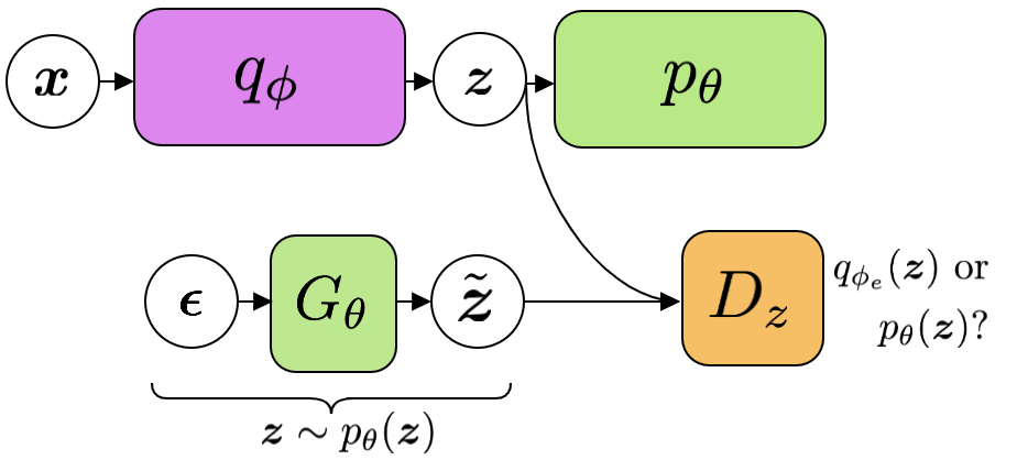
Concretely, we could learn a kind of VAE where the per-example KL term is instead replaced with an `adversarial' divergence \(\fdiv\) 5 between \(\qp(\ZZ)\) and a learnable prior \(\ptgreen(\ZZ)\) (Figure X):
\begin{align} \label{eq:cvae:adv_ae} \min_{\thetagr, \phip} \ -\mathbb{E}_{\qp(\zz,\xx)} \log \pt(\xx|\zz,\yy) + \lambda \fdiv \Big[ \qp(\ZZ) \| \pt(\ZZ) \Big], \tag{16} \end{align}where samples \(\zz \sim \ptgreen(\zz)\) are computed via \(\zz = G_{\theta}(\eta)\) for some simple prior \(p(\eta)\). While equation \ref{eq:cvae:adv_ae} is no longer an ELBO, one can think of there existing an actual ELBO which is just the likelihood term plus the per-example KL between \(\qp(\XX|\ZZ,\YY)\) and \(\ptgreen(\ZZ)\), which in our case is not computable in closed form since \(\ptgreen(\zz)\) is implicitly represented by the generator.
While this is an interesting start, one issue is that samples from the learned prior may not necessarily decode into plausible looking samples. For instance, if \(\qp(\zz)\) is not sufficiently smooth but rather 'spiky', then samples from \(\ptgreen(\zz)\) which don't fall into one of those spikes may not decode into a plausible image. In such a case, we may need to add extra regularisation in the form of an \emph{additional} adversarial loss which ensures that decoded samples from \(\ptgreen(\xx)\) should be indistinguable from those from the real data distribution \(q(\xx)\). In that case, we should really be training a GAN to match the generative and inference pathways:
\begin{align} \label{eq:cvae:adv_ae_joint} \min_{\thetagr, \phip} \ -\mathbb{E}_{\qp(\zz,\xx)} \log \ptgreen(\xx|\zz,\yy) + \fdiv \Big[ \qp(\ZZ, \XX) \| \ptgreen(\ZZ, \XX) \Big]. \tag{16} \end{align}
It turns out that Eqn. (17) without the likelihood term is equivalent to the bidirectional GAN (dumoulin2016adversarially, donahue2016adversarial). In particular, these models propose the following loss:
However, one downside is the learned inference encoder \(\qp(\zz|\xx)\) is inaccurate and cannot be used to faithfully reconstruct examples, due to the fact that there is no explicit reconstruction (likelihood) loss. As mentioned in dumoulin2016adversarially however one could learn a separate encoder in a post-hoc fashion to address this issue. This issue is also addressed in li2020decomposed.
4.1. cVAEs and conditional Gaussian diffusion models
Diffusion models can be seen as multi-latent generalisations of VAEs ho2020diffusion, and are theoretically very closely related to score-based generative models (see weng2021diffusion for derivations showing their equivalence for the case where the distributions are Gaussian). Instead of just a single latent variable \(\zz\), we have many noisy versions of \(\xx\) which we denote \(\xx_1, \dots, \xx_T\) for \(T\) denoising diffusion timesteps (but we can think of this collection of as variables as just \(\zz\) for convenience). Apart from this, the main differences are:
- There is no inference network \(\qp\), instead \(q\) is fixed and we have a joint distribution which is the forward process \(q(\xx_0, \dots, \xx_T)\) where larger \(t\) corresponds to progressively noisier data;
- all \(\xx_t\) for \(t \in \{1, \dots, T\}\) are the same dimension as \(\xx_0\);
- and \(q(\xx_T|\xx_{t-1}) \approx q(\xx_T)\) for sufficiently large total number of timesteps \(T\), and we denote the prior \(p(\zz) = q(\xx_T)\).
As for conditional diffusion models, some commonly used variants of diffusion are not derived from the conditional ELBO. They're usually modifications done to the reverse conditional to also condition on \(\yy\), to give \(\pt(\xx_{t-1}|\xx_t, \yy)\). If we denote the collection of noisy random variables \(\xx_1, \dots, \xx_T\) as just \(\zz\), we can think of that sort of model's decoder as \(\pt(\xx|\zz,\yy)\) instead of \(\pt(\xx_0|\xx_1, \dots, \xx_T, \yy)\). Therefore, these formulations can be seen as fancier \(\ZZ,\YY\) dependent VAEs. To the best of my knowledge, I have not seen a formulation analogous to the \(\ZZ,\YY\) independent case.


5. Conclusion
In conclusion, we have:
- Derived conditional VAEs through the lens of minimising the KL divergence between two distributions: the inference and generative distributions, which comprise the two halves of a variational autoencoder.
- Introduced two conditional variants, corresponding to whether \(\ZZ\) and \(\YY\) are independent and dependent. For the independent case, we highlighted its usefulness in controllable generation.
- Discussed the need to carefully balance the weight of the KL term, which balances the trade-off between sample quality and coverage with respect to the inference and generative distributions. We also derived a mutual information based interpretation of the KL term in order to elucidate its effect on training.
- Presented experiments on toy 2D datasets which corroborate our theoretical observations.
- Discussed how one can avoid the difficulty of optimising a VAE by instead training an adversarial autoencoder and learning a prior distribution to match the inference marginal. From this discussion we arrive at the bidirectional GAN, which has a very close relationship with the VAE in the sense that the former minimises an arbitrary \(f\) divergence between the generative and inference pathways while the latter uses the forward KL divergence. This brings us full circle!
6. Appendix
6.1. Derivation of Esmaeli's joint KL
Here we derive the main equation presented in esmaeili2018structured. This corresponds to the unconditional VAE, without \(\yy\) conditioning.
where:
- \(\ptgreen(\xx) = \int_{\zz} \ptgreen(\xx|\zz)p(\zz) d \zz\), the marginal distribution of the data with respect to the generative process. This is also called the marginal likelihood.
- \(\qp(\zz) = \int_{\xx} \qp(\zz|\xx)q(\xx) d\xx\) , the marginal distribution over the latent code with respect to the inference process. This is also called the inference marginal.
6.2. Conditional case
We can derive the conditional case by adding \(\yy\) wherever it is necessary. Starting from Eqn. (10f), we derive the following:
\begin{align} & \mathbb{E}_{\qp(\zz,\xx,\yy)} \Big[ \log \frac{\ptgreen(\xx|\zz,\yy)}{\ptgreen(\xx)} - \log \frac{\qp(\zz|\xx,\yy)}{\qp(\zz)} \Big] + \mathbb{E}_{q(\xx)} \Big[ \log \frac{\ptgreen(\xx)}{q(\xx)} \Big] + \mathbb{E}_{\qp(\zz,\yy)} \Big[ \log \frac{p(\zz,\yy)}{\qp(\zz)} \Big]. \tag{11a} \end{align}We can subsequently refine this equation depending on the factorisation of \(p(\zz,\yy)\), which we do below.
6.2.1. z and y are independent
For the sake of space, I will simply use \(\qp\) to refer to the full joint distribution \(\qp(\zz,\xx, \yy)\). For \(p(\zz,\yy) = p(\zz)p(\yy)\), we get:
\begin{align} & \mathbb{E}_{\qp} \Big[ \log \frac{\ptgreen(\xx|\zz,\yy)}{\ptgreen(\xx)} - \log \frac{\qp(\zz|\xx,\yy)}{\qp(\zz)} \Big] + \mathbb{E}_{q(\xx)} \Big[ \log \frac{\ptgreen(\xx)}{q(\xx)} \Big] + \\ & \ \ \ \ \ \mathbb{E}_{\qp(\zz,\yy)} \Big[ \log \frac{p(\zz)}{\qp(\zz)} + \log p(\yy) \Big] \tag{12a} \\ & = \mathbb{E}_{\qp} \Big[ \log \frac{\ptgreen(\xx|\zz,\yy)}{\ptgreen(\xx)} - \log \frac{\qp(\zz|\xx,\yy)}{\qp(\zz)} \Big] + \mathbb{E}_{q(\xx)} \Big[ \log \frac{\ptgreen(\xx)}{q(\xx)} \Big] + \\ & \ \ \ \ \ \mathbb{E}_{\qp(\zz)} \Big[ \log \frac{p(\zz)}{\qp(\zz)} \Big] + \mathbb{E}_{q(\yy)} \log p(\yy) \tag{12b} \\ & = \mathbb{E}_{\qp} \Big[ \underbrace{\log \frac{\ptgreen(\xx|\zz,\yy)}{\ptgreen(\xx)}}_{\circleone} - \underbrace{\log \frac{\qp(\zz|\xx,\yy)}{\qp(\zz)}}_{\circletwo} \Big] - \underbrace{\kldiv\Big[ q(\XX) \| \ptgreen(\XX) \Big]}_{\circlethree} \\ & \ \ \ \ \ - \underbrace{\kldiv\Big[ \qp(\ZZ) \| p(\ZZ)}_{\circlefour} \Big] + \text{const.} \tag{12c} \end{align}Here, \(p(\yy)\) can fall out of the optimisation since it's just a constant. However, since it's a prior we can set it to whatever it is we want it to be, either the actual empirical distribution of \(\yy\) for our dataset or another distribution.
6.2.2. z and y are dependent
Again, starting from Eqn. (10f), if we assume that \(p(\zz,\yy) = p(\zz|\yy)p(\yy)\) then:
\begin{align} & \mathbb{E}_{\qp(\zz,\xx,\yy)} \Big[ \log \frac{\ptgreen(\xx|\zz,\yy)}{\ptgreen(\xx)} - \log \frac{\qp(\zz|\xx,\yy)}{\qp(\zz)} \Big] + \mathbb{E}_{q(\xx)} \Big[ \log \frac{\ptgreen(\xx)}{q(\xx)} \Big] + \\ & \ \ \ \ \mathbb{E}_{\qp(\zz,\yy)} \Big[ \log \frac{p(\zz|\yy)p(\yy)}{\qp(\zz)} \Big] \tag{13a} \\ & \mathbb{E}_{\qp(\zz,\xx,\yy)} \Big[ \log \frac{\ptgreen(\xx|\zz,\yy)}{\ptgreen(\xx)} - \log \frac{\qp(\zz|\xx,\yy)}{\qp(\zz)} \Big] + \mathbb{E}_{q(\xx)} \Big[ \log \frac{\ptgreen(\xx)}{q(\xx)} \Big] + \\ & \ \ \ \ \mathbb{E}_{\qp(\zz,\yy)} \Big[ \log \frac{p(\zz|\yy)}{\qp(\zz)} + \log p(\yy) \Big]. \tag{13b} \\ & \mathbb{E}_{\qp(\zz,\xx,\yy)} \Big[ \log \frac{\ptgreen(\xx|\zz,\yy)}{\ptgreen(\xx)} - \log \frac{\qp(\zz|\xx,\yy)}{\qp(\zz)} \Big] - \kldiv\Big[ q(\XX) \| \ptgreen(\XX) \Big] + \\ & \ \ \ \ -\kldiv \Big[ \qp(\ZZ) \| p(\ZZ|\YY) \Big] + \mathbb{E}_{q(\yy)} \log p(\yy). \tag{13c} \\ \end{align}Here, we need to choose what \(p(\zz|\yy)\) is. Either it can be a fixed distribution (i.e. a distribution is pre-assigned for each possible value of \(\yy\)), or it could also be learned, in which case we can denote it as \(\ptgreen(\zz|\yy)\).
6.3. Per-example KL versus marginal KL
Thanks to Eqn. (10e) we can just re-arrange its terms to express their relationship as the following:
\begin{align} \kldiv \Big[ \qp(\ZZ|\XX,\YY) \| p(\ZZ|\YY) \Big] - I_{\phip}(\ZZ; \XX, \YY) = \kldiv[ \qp(\ZZ) \| p(\ZZ|\YY) ] + \text{const.} \tag{10e} \end{align}Therefore, minimising the marginal KL on the RHS of this equation means:
- (1) Making \(I\) larger, for a fixed per-example KL (first term on the LHS);
- (2) or making per-example KL smaller, for fixed \(I\).
(1) seems beneficial because increasing \(I\) means \(\ZZ\) loses less information about \(\XX\), but this only makes sense in the context of a \(\ZZ,\YY\) dependent VAE.
We also note the RHS of this equation was proposed in kumar2017variational, but for unconditional VAEs.
6.4. Z-Y independent cVAE on SVHN
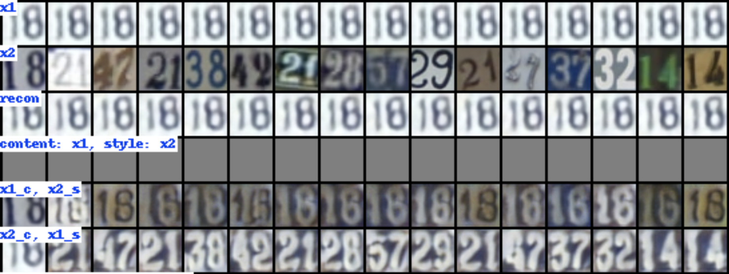
Here is an artifact from an old research project I did involving controllable generation. We were trying to do style/content swaps for images from SVHN – here, one can think of the content as being \(\yy\), the identity of the SVHN digit. For each row:
x1is \(\xx_1\),x2is \(\xx_2\). Their corresponding labels are the digits, e.g. \(\yy_1\) will be 18. \(\yy_2\) depends on what column we are looking at.reconis the reconstruction of \(\xx_1\), as per the inference process.x1_c, x2_ssays: take the content of \(\xx_1\) and the style from \(\xx_2\). This means, we sample \(\xx \sim \ptgreen(\xx|\yy_1,\zz_2)\), where \(\yy_1\) is the identity of \(\xx_1\), and \(\zz_2 \sim \qp(\zz|\yy_2,\xx_2)\).x2_c, x1_ssays the opposite: take the content of \(\xx_2\) and the style from \(\xx_1\). This means, we sample \(\xx \sim \ptgreen(\xx|\yy_2,\zz_1)\), where \(\yy_2\) is the identity of \(\xx_2\), and \(\zz_1 \sim \qp(\zz|\yy_1,\xx_1)\).
7. References
beckham2023thesisBeckham, C. (2023). PhD thesis dissertation. (Work in progress.)kingma2013autoKingma, D. P., Welling, M., & others, (2019). An introduction to variational autoencoders. Foundations and Trends in Machine Learning, 12(4), 307–392.kingma2019introductionKingma, D. P., Welling, M., & others, (2019). An introduction to variational autoencoders. Foundations and Trends in Machine Learning, 12(4), 307–392.esmaeili2018structuredEsmaeili, B., Wu, H., Jain, S., Bozkurt, A., Siddharth, N., Paige, B., Brooks, D. H., … (2018). Structured disentangled representations. arXiv preprint arXiv:1804.02086, (), .burgess2018understandingBurgess, C. P., Higgins, I., Pal, A., Matthey, L., Watters, N., Desjardins, G., & Lerchner, A. (2018). Understanding disentangling in beta-VAE. arXiv preprint arXiv:1804.03599, (), .child2020veryChild, R. (2020). Very deep VAEs generalize autoregressive models and can outperform them on images. International Conference on Learning Representations, (), .ho2020diffusionHo, J., Jain, A., & Abbeel, P. (2020). Denoising diffusion probabilistic models. Advances in Neural Information Processing Systems, 33(), 6840–6851.dhariwal2021diffusionDhariwal, P., & Nichol, A. (2021). Diffusion models beat GANs on image synthesis. Advances in Neural Information Processing Systems, 34(), 8780–8794.kumar2017variationalKumar, A., Sattigeri, P., & Balakrishnan, A. (2017). Variational inference of disentangled latent concepts from unlabeled observations. arXiv preprint arXiv:1711.00848, (), .dumoulin2016adversariallyDumoulin, V., Belghazi, I., Poole, B., Lamb, A., Arjovsky, M., Mastropietro, O., & Courville, A. (2016). Adversarially Learned Inference. In , International Conference on Learning Representations (pp. ). : .donahue2016adversarialDonahue, J., Kr\"ahenb\"uhl, Philipp, & Darrell, T. (2016). Adversarial feature learning. arXiv preprint arXiv:1605.09782, (), .nowozin2016fNowozin, S., Cseke, B., & Tomioka, R. (2016). F-gan: training generative neural samplers using variational divergence minimization. Advances in neural information processing systems, 29(), .zhang2019variationalZhang, M., Bird, T., Habib, R., Xu, T., & Barber, D. (2019). Variational f-divergence minimization. arXiv preprint arXiv:1907.11891, (), .makhzani2015adversarialMakhzani, A., Shlens, J., Jaitly, N., Goodfellow, I., & Frey, B. (2015). Adversarial autoencoders. arXiv preprint arXiv:1511.05644, (), .larsen2016autoencodingLarsen, A. B. L., S\onderby, S\oren Kaae, Larochelle, H., & Winther, O. (2016). Autoencoding beyond pixels using a learned similarity metric. In , International conference on machine learning (pp. 1558–1566). : .mescheder2017adversarialMescheder, L., Nowozin, S., & Geiger, A. (2017). Adversarial variational bayes: unifying variational autoencoders and generative adversarial networks. In , International conference on machine learning (pp. 2391–2400). : .chen2016infoganChen, X., Duan, Y., Houthooft, R., Schulman, J., Sutskever, I., & Abbeel, P. (2016). InfoGAN: interpretable representation learning by information maximizing generative adversarial nets. Advances in neural information processing systems, 29(), .van2017neuralVan Den Oord, A., Vinyals, O., & others, (2017). Neural discrete representation learning. Advances in neural information processing systems, 30(), .goodfellow2020generativeGoodfellow, I., Pouget-Abadie, J., Mirza, M., Xu, B., Warde-Farley, D., Ozair, S., Courville, A., … (2020). Generative adversarial networks. Communications of the ACM, 63(11), 139–144.
Footnotes:
One may wonder whether it is more appropriate to instead modify the KL term to be less 'strict' and match \(\qp(\ZZ|\YY)\) with \(p(\ZZ)\) instead, and we discuss this in Sec. 6.3.
While it is possible in principle to derive an additional loss term which specifically penalises \(I(Z; Y)\) (e.g. with Monte Carlo approximation or with adversarial learning), from personal experience it came with very little success. I suspect it is because such a term only works if the likelihood term is sufficiently downweighted, but this causes sample quality to suffer and we just end up with the same problem as we do with the original KL term.
If one had a highly supervised dataset of 'paired' examples \((\xx^{(i)}_1, \xx^{(i)}_2)\) where \(\xx_1\) and \(\xx_2\) only dithered by \(\YY\) (i.e. all other factors of variation remained the same) then it would perhaps be much easier to learn this style of VAE, but such datasets are usually not reflective of the real world.
Interestingly, another mutual information term falls out of the derivation and it is negative. Since Eqn. (14f) is framed as a minimisation, minimising the negative of this is really maximising it, so \(\phip\) is also being updated to maximise the mutual information between \(\ZZ\) and \(\YY\) with respect to the encoder \(\qp\).
The tilde emphasises that GANs are approximating a particular $f$-divergence, see goodfellow2020generative.