Vicinal distributions as a statistical view on data augmentation

What \(\pt(y|\xx)\) is depends on the particular distribution that is assumed, which depends on the data. For instance, if we are performing maximum likelihood on a discrete classification task, then we assume that the \(\pt(y|\xx)\) is a categorical distribution. That is:

where \(\ft(\xx) \in [0,1]^{k}\) is a probability distribution over the \(k\) classes and \(\sum_{j} \ft(\xx)_j = 1\).

If \(y \in \{0, 1\}^{k}\) is a one-hot label over \(k\) classes and \(\ft(\xx) \in [0,1]^{k}\) (whose vector sums to 1) then we can simply write the log likelihood as:

where \(c(y_i)\) indexes into the correct class. While this is usually the case that ground truth labels are one-hot, it may not be the case in certain other situations. In fact, we will see later on that Equation (2) is needed for one of the augmentations we consider.

One can also derive log likelihoods for the binary classification and regression cases, and these correspond to \(\pt\) being either a Bernoulli or Gaussian distribution, respectively. To keep things general however, we will simply stick to Equation (1) as this abstracts away having to think about what distribution is being used for \(\pt\).

From the point of view of optimisation and nothing else, Equation (1) is what we would like to maximise. In practice however, we probably don't want to do this because we run the risk of overfitting to the training set. This is the same reason why the issue of local minima for deep neural networks isn't always a big deal, because being at the lowest local minima is probably not going to give good generalisation performance.

What we really want to do is to compute Equation (1) but over a held-out validation set which has not been trained on, \(\Dvalid\). Assuming we have trained \(m\) models via Equation (1) (one for each hyperparameter or seed), we would like to find the best weights \(\tbest \in \Theta = \{ \theta_j \}_{j=1}^{m}\) such that the log likelihood is maximised but over the validation set:

It is also possible to consider other validation metrics to measure over the validation set. Whichever one is used depends on the particular problem domain considered. Here, we have decided to keep things simple and use a validation metric that is the same as the training loss, but computing accuracy over the validation set is reasonable as well.

The vicinal distribution \(\tilde{p}(\xxt, \yt|\xx,y)\) can be further simplified depending on the assumptions made on the relationship between the images and labels. For instance, many data augmentations only operate on the input \(\xx\) and ignore the label. In that case the vicinal distribution simplifies down to:

and \(\delta(\yt=y)\) is the dirac function, i.e. all of its probability mass is centered on \(y\). Equation (7) is a label preserving data augmentation, since it is assumed that whatever we do to \(\xx\) will not change its semantic meaning with respect to the label considered.

Let us discuss a few more types of factorisations:

• \(p(\xxt, \yt|\xx,y) = \delta(\xxt = \xx)p(\yt|y)\), i.e. the original image is preserved but the label changes. An example of this is the label smoothing technique (szegedy2016rethinking), which suggests that a one-hot label have noise added to it such that every other non-correct class in the distribution has mass \(\epsilon\).
• \(p(\xxt, \yt|\xx,y) = p(\xxt|\xx, y)p(\yt|y)\). One example of this pertains to defending against adversarial examples. For the sake of brevity, rather than a formal definition we can simply say that an adversarial example is one that 'fools' a classifier in a rather non-intuitive way. One such instance is an image that unambigiously belongs to class \(y\) but with imperceptible noise added \(\eta \in \mathbb{R}^{d}\) such that the classifier assigns it \(y' \neq y\) with extremely high confidence (goodfellow2014explaining). The 'fast gradient sign method' – FGSM – can find such potential adversarial inputs under one optimisation step, assuming that it is possible to compute gradients wrt to the classifier. This can be framed as one optimisation step \(\xxt := \xx + \epsilon \cdot \sgn(\nabla_{\xx} \log \pt(\xx|y))\), where \(\epsilon\) is a very small scalar, and possibly even a random variable. Therefore, FGSM can be seen as a vicinal distribution of the form \(p(\xxt|\xx,y)\delta(\yt = y)\).

In the next section we will discuss a very interesting type of vicinal distribution, one which can be seen as a generalisation of \(\pt(\xxt, \yt | \xx, y)\).

An interesting class of data augmentations, called mixup, proposes the generation of augmented examples by considering convex combinations of pairs of real examples. That is, given two pairs \((\xx_1, y_1) \sim p(\xx, y)\) and \((\xx_2, y_2) \sim p(\xx, y)\) as well as a mixing coefficient \(\lambda \sim \text{Beta}(\alpha, \alpha)\) , a linear combination between the two pairs of inputs is computed as:

and these are used in conjunction with Equation (2) to define the training loss. (Note that we cannot use Equation (2a) since the resulting labels \(\yt\) are no longer guaranteed to be one-hot vectors.)

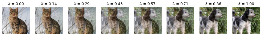
In Figure 2 we show examples of mixup-produced images between two images, one of a cat and one of a dog. The images are produced with \(\lambda\xx_{\text{dog}} + (1-\lambda)\xx_{\text{cat}}\), and the values of \(\lambda\) are shown above each image.

Despite the fact that most of these images do not look representative of the data distribution – with the smaller-weighted image 'ghosting' the higher weighted image – there is ample empirical evidence to suggest such images work well in practice as a form of data augmentation. One intuitive explanation for this is that the interpolated label \(\yt\) does confer useful information given the interpolated image \(\xxt\), even if it doesn't look plausible. For instance, if we mix an image of a cat and a dog with a mixing ratio of 50% (i.e. \(\lambda = 0.5\)) then it makes sense for the corresponding label to be \([0.5, 0.5]\), rather than either \([1,0]\) or \([0,1]\). Another intuition is that mixup acts as a form of regularisation that specifically encourages \(\ft\) to behave linearly in between training examples, and this is qualitatively demonstrated in zhang for toy datasets in 2D. While these explanations may not be sufficient for the more mathematically inclined reader, we defer them to carratino2020mixup, which presents a rigorous theoretical analysis into why mixup works well in practice.

Since the mixing function is stochastic, we can write it out as a vicinal distribution of the form:

and therefore the joint distribution over all the concerned variables becomes:

The mixup training objective becomes:

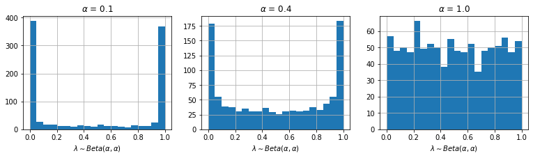
One hyperparameter that mixup introduces is \(\alpha\), which controls the shape of the beta distribution. The authors note that \(\alpha \in [0.1, 0.4]\) give the best results, and that \(\alpha = 1.0\) is more likely to overfit. When we plot their histograms in Fig. 3, we can see that \(\alpha \in [0.1, 0.4]\) gives a distribution over \(\lambda\) such that it is either close to one or zero. This would have the effect of minimising on the average the number of 'ghost' images produced, since these look most unusual with respect to the real data distribution. Conversely, \(\alpha = 1.0 \implies \text{Uniform}(0,1)\), and all values of \(\lambda\) are equally likely to be sampled.

Lastly, while the mixing function in Eqn. (5) is simply a linear combination between the pairs of inputs, other varieties include superimposing parts of images together, or even performing linear combinations in the latent space of a classifier (verma2019manifold).

Lastly, we note that one limitation of most mixup approaches is that the mixes are generated in input space, which limits the space of interesting transformations one can do to the data. Performing mixup in latent space is a way around that, because the image is being manipulated at a higher level of abstraction than just individual pixels. One of the contributing publications of this thesis is in some work we did that proposed exactly this, but in the context of unsupervised learning.

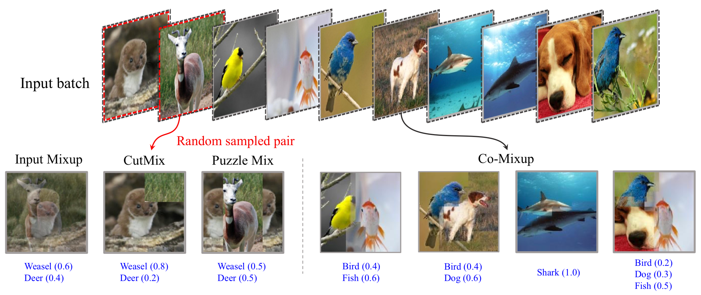
Figure 2 (attribution: CoMixup kim2021co) shows a range of mixing functions defined in input space. The left-most example shown in this figure, input mixup, is the algorithm described in Equations (5) and (5b). The second left-most function, CutMix, proposes superimposing a random crop of one image on top of another. Lastly, more sophisticated variants of this exist, whose details we defer to kim2021co.

What is interesting about mixup is that – unlike in Eqn. (4) – the vicinal distribution here is being conditioned on two pairs of \((\xx,y)\) inputs. In principle however, nothing is stopping us from conditioning on any arbitrary collection of pairs, and so mixup in a sense can be thought of as implementing the following vicinal distribution:

where \(\mathbf{X} =\{ (\xx_i, y_i) \}_{j=1}^{m}\) for \(m\) input/output pairs from the ground truth distribution. Since the vicinal distribution \(\tilde{p}_{\text{mix}}\) can also internally encapsulate any kind of single-example data augmentation trick, we can think of mixup as actually generalising all of the data augmentation techniques that we've presented so far: if \(m = 1\) then we get data augmentation algorithms that operate on a single example, and if \(m > 1\) we get mixup-style algorithms.