A somewhat mathematical introduction to Gaussian and Laplace autoencoders

@misc{beckhamc_intro_ae,
  author = {Beckham, Christopher},
  title = {A statistical introduction to Gaussian and Laplace autoencoders},
  year = {2021},
  publisher = {GitHub},
  journal = {GitHub repository},
  howpublished = {\url{https://beckham.nz/2021/06/28/training-gans.html}}
}

In this blog post, I will:

• Provide a statistically grounded introduction to deterministic autoencoder (AE) by relating its most commonly used loss function (the mean squared error between the input and reconstruction) to the maximisation of a Gaussian likelihood.
• Show that typical implementations of AE fix the variance to a scalar constant, but also show how it can be learned to achieve higher likelihoods on the data.
• Derive gradients for different formulations of a Gaussian autoencoder, and suggest why I think you should use the Laplace distribution, which is closely related to Gaussian.
• (Coming soon) Provide some code which allows you to easily train a Gaussian or Laplacian VAE on MNIST. This code leverages PyTorch’s torch.distributions module which heavily eases implementation of variational methods.

Updates:

• (29/09/2021) Fix minor errors in derivations, make clearer the derivation of multivariate Gaussian likelihood.
• (22/08/2021) Provide minimalistic code to implement the AE/VAE forward pass with torch.distributions.
• (18/08/2021) Thanks Vikram Voleti for pointing out numerous errors: (1) error where the numerator for the log RMSE gradient was incorrectly being multiplied by 2; and (2) Fig 4’s plot not being consistent with its equation.

Table of contents

• Deriving mean squared error from a Gaussian distn.
  • Deconstructing the Gaussian distribution
  • Modelling the variance
  • Extra stuff: modelling more than one variance
• Laplace output distribution and the L1 norm
  • Example: variational autoencoders
• Code
  • Minimalistic forward pass of an AE / VAE
• References

Deriving mean squared error from a Gaussian distn.

The most basic autoencoder, which I will refer to as the ‘deterministic’ autoencoder (AE), simply involves constructing an encoder and decoder network and minimising the L2 distance between the input and its reconstruction, otherwise known as the reconstruction error. For some input \(\mathbf{x} \in \mathbf{R}^{n}\):

where \(f_{\theta}\) denotes the encoder, \(g_{\theta}\) denotes the decoder, and \(\mathbf{x}\) is the input. Since we’re dealing with images for this blog post, we can think of \(\mathbf{x}\) as being the flattened 2D matrix of dimension $(h, w)$, denoting the height, and width, respectively. Here, we want to find a latent code \(\mathbf{z} = f_{\theta}(\mathbf{x}) \in \mathbf{R}^{p}\) of dimension \(p << n\), where \(p = h \times w\) is the total dimensionality of the input. For RGB images, \(\mathbf{x}\) will of course have an extra dimension corresponding to the channel, but we will keep things simple here.

Since the latent dimension \(p\) is much smaller than the data dimension \(n\), the intuition is that this will constrain the network to only learn the most salient features in order to reconstruct the data. In this vein, we can think of autoencoders essentially performing learning via compression. The loss here should be quite intuitive: we want to minimise some distance between the real input and its reconstructed version, with the distance here chosen to be the L2 norm. The reason for the L2 norm can be explained if we view the autoencoder through a more probabilistic lens: denoting \(z = f_{\theta}(\mathbf{x})\), we would like to model \(p(\mathbf{x}|\mathbf{z})\), otherwise known as the likelihood. It turns out that this likelihood is derived by assuming the output (reconstruction) of the autoencoder is a draw from a Gaussian distribution:

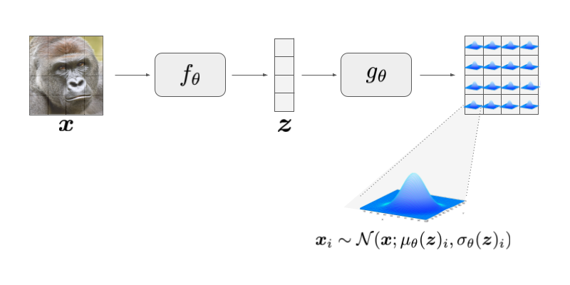
where the mean \(\mu_{\theta}(\mathbf{x})\) and covariance \(\sigma_{\theta}(\mathbf{z})\) are functions modelled by deep nets, and Gaussian modelled has independent dimensions, corresponding to a diagonal covariance matrix. Note that since this is an independent Gaussian, each dimension of \(\mathbf{x}\) is conditionally independent given \(\mathbf{z}\), i.e. \(p(\mathbf{x}|\mathbf{z}) = \prod_{i=1}^{n} p(\mathbf{x}_{i}|\mathbf{z})\), where the product is over the \(n\) dimensions of \(x\) (e.g. 784 for a 1x28x28 pixel image). This means we can simply model the likelihood of each individual pixel as the following:

For the sake of simplicity, for most of this section I will use a non-boldfaced \(x\) to refer to any arbitrary pixel in an image \(\mathbf{x}_{i}\). Once we understand what is happening with any arbitrary pixel \(x\) we can easily generalise it to all of the pixels in the input image.

This new notation – the use of \(\mu(\cdot)\) and \(\sigma(\cdot)\) as functions – differs slightly from Equation(1) and Figure (1): \(\mu_{\theta}(z)\) and \(\sigma_{\theta}\) can be thought of as two functions that branch from the end of \(g_{\theta}(z)\). These model the means and variances of the individual pixels in the output, as shown in Fig 1.

Deconstructing the Gaussian distribution

We will revisit this shortly. For now, let’s take a look at the Gaussian pdf for a single pixel \(x\), which is as follows:

Since we’d like to derive the log likelihood, taking the log and expanding out the partition function yields us:

Substituting \(\sigma\) for \(\sigma(z)\) and \(\mu\) for \(\mu(z)\), and removing the constant term, we define the log-likelihood (for a single example \(x\)) as:

Since we typically perform minimisations over loss functions in DL frameworks, let us take the negative, so we get the negative log-likelihood (NLL):

Let us now consider a vector \(\mathbf{x}\) (which you could think of as the flattened 2D matrix which represents the input image). For a multivariate Gaussian that is isotropic (i.e. each dimension has the same variance and dimensions are independent), we can simply define the NLL as the sum of the NLL of the individual pixels:

where \(\mathbf{z} = f_{\theta}(\mathbf{x})\). Such an expression can also be derived easily by taking the equation of a multivariate Gaussian that is defined by a mean vector \(\boldsymbol{\mu}\) and covariance matrix \(\boldsymbol{\Sigma}\) and working ‘backwards’ to obtain the above derivation. Let me do one last thing, which is multiply by sides by \(\frac{1}{n}\) so that we instead have a mean squared error rather than a sum of squared errors:

Typically with autoencoders, the variance term is assumed to be fixed to \(\sigma_{z}^2=1\) across all dimensions. In other words, for Equation (2) \(\text{diag}(\sigma(\mathbf{z}))_{i} = \sigma_{z}\) for all \(i\). This means that the first term for Equation (5) cancels out (\(\log(1) = 0\)) which yields us the mean squared error (MSE) loss:

This is typically what is written in most autoencoder implementations. Finally, we minimise such a loss over our training set of examples \(\{ \mathbf{x}^{(j)} \}_{j=1}^{m}\), where the superscript in parentheses \(\mathbf{x}^{(j)}\) signifies the \(j\)‘th training example:

Since we’re doing this all in the context of deep learning, the above loss is approximated with SGD via the use of minibatches.

Modelling the variance

Let’s consider a univariate Gaussian once again (remembering that the multivariate case is really just a sum over univariate distributions, as illustrated by equation (4)):

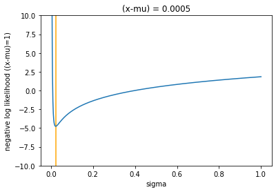
We can see that the numerator is being divided by the variance term. What is interesting is that this particular likelihood function is unbounded : if we fix the numerator \((x-\mu)^2\) to some constant \(K\) and examine the function with respect to \(\sigma\), the output tends to \(\infty\) as \(\sigma \rightarrow 0\). We can illustrate this by plotting.

import numpy as np
import matplotlib.pyplot as plt
%matplotlib inline

def gaussian(start_x, end_x, K, ylim_min=-10, ylim_max=10):
    """
    Parameters
    ----------
    
    K: K = (x - \mu)^2
    """

    sigma = np.linspace(start_x, end_x, num=1000)
    
    # test: implement actual pdf then take log of it to verify
    #ll = np.log( 1.0 / (sigma*np.sqrt(2*np.pi)) * np.exp(  -0.5 * (K**2 / sigma)  ) )
    #nll = -ll
    
    nll = np.log(2*np.pi*(sigma**2)) + (K/(sigma**2))

    plt.plot(sigma, nll)
    plt.xlabel('sigma')
    plt.ylabel('negative log likelihood ((x-mu)=1)')
    plt.ylim(ylim_min, ylim_max)
    plt.title("(x-mu) = {}".format(K))
    plt.vlines(np.sqrt(K), ylim_min, ylim_max, colors="orange")

# assume reconstruction error (x-mu)**2 is 0.0001
gaussian(1e-5, 1, K=0.0005)

# assume reconstruction error (x-mu)**2  is almost zero, 0.000001
gaussian(1e-7, 1, K=1e-10, ylim_max=20, ylim_min=-20)

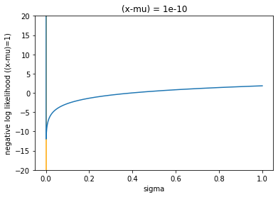
In both plots, I have marked the value of \(\sigma\) that minimises the function, which is shown as an orange vertical bar. This paper [#ref:vae_yu] was an interesting read, and basically states that simplifying the likelihood to squared error is suboptimal, and that, for a fixed MSE the \(\sigma\) that actually minimises the NLL is \(\sqrt{2\text{MSE}}\) plus a constant term. This can be proven with some simple calculus, taking the derivative of the NLL, setting it to zero, and solving for \(\sigma\). For the first term:

where I have re-written \(\log(\sqrt{2 \pi} \sigma) = \log(\sqrt{2 \pi \sigma^2}) = \log( (2 \pi \sigma^2)^{\frac{1}{2}} ) = \frac{1}{2} \log(2 \pi \sigma^2)\).

And the second:

Summing the two gradient terms together give us:

Setting this expression to zero and solving for \(\sigma\):

Plugging this into Equation (4):

hence, we get the log root mean squared error (well, the log root of twice the MSE). Why is this interesting? How does it differ from the regular mean squared error? We can gain some insights by computing the gradient. Here I am going to use Sympy which is a symbolic math library which allows one to compute derivatives and pretty print them – this is great for verifying that your manually-computed derivatives are correct:

from sympy import *

def verify_gradient():
    # Compute log(MSE), where the sum of squares is simply
    # two terms (x1-y1)**2 + (x2-y2)**2.
    x1, y1, x2, y2, n = symbols('x1 y1 x2 y2 n')
    return simplify(
        diff(
            log( sqrt((1/n) * ( (x1-y1)**2 + (x2-y2)**2 )) ),
            x1
        )
    )

verify_gradient()

It’s worth mentioning that ommitting the square root here simply multiplies the gradient by 2 (you can verify this by removing the sqrt call in verify_gradient), so from now on I will call this the log mean squared error since it really doesn’t change anything. To re-write the gradient more formally:

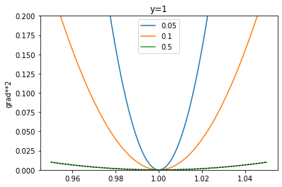
Since the SSE (sum of squared errors) is sitting in the denominator, as it decreases in magnitude and the total sum is < 1, the resulting gradient starts to become larger. By re-writing the denominator to \((x_i-y_i)^2 + \delta\) where \(\delta = \sum_{j \neq i}(x_j - y_j)^2\), we can plot the gradient for different values of \(\delta\) as well as compare to MSE, shown as a dotted black line:

xs = np.linspace(0.95,1.05,num=1000)
deltas = [0.05, 0.1, 0.5]
for delta in deltas:
    # assume y=1 here
    ys = (xs-1) / ( (xs-1)**2 + delta )
    plt.plot(xs,ys**2)
plt.ylabel('grad**2')
plt.title('y=1')
plt.ylim(0, 0.2)
#plt.ylim(-1, 20)
plt.legend(deltas)

ys_mse = 2*(xs - 1.)
plt.plot(xs,ys_mse**2, c="black", linestyle="dotted")

Interesting observation I made: there needs to be a mean over the \((x_i - y_i)^2\) terms for this loss to make sense. For instance, if we were to minimise the log squared error rather than mean squared error , then the gradient of the loss w.r.t. \(x\) would be:

This derivative is just a few steps of the chain rule so it’s not too hard, but let’s just verify it anyway with sympy because I like to use it:

def verify_gradient():
    # Compute log(MSE), where the sum of squares is simply
    # one term (x1-y1)**2.
    x1, y1, n = symbols('x1 y1 n')
    return simplify(
        diff( 
            log( (1/n) * ( (x1-y1)**2 ) ), 
            x1
        )
    )

verify_gradient()

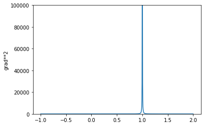
The magnitude of the gradient actually tends to infinity (explodes) as \(\vert x-y \vert\) approaches zero. This is completely different behaviour to what we would expect intuitively, which is that the magnitude of the gradient should be decreasing to zero as \(|x-y|\) decreases.

This means that if you were training, say, a linear regression with SGD for a batch size of 1 and minimising the loss \(\log (x-y)^2\) training would not converge! Note that this would simply not happen for the regular squared error \((x-y)^2\) loss. If you’re using minibatches however, the resulting loss would be simply a mean over the \(m\) examples in the minibatch \(\frac{1}{m} \sum_{j} \log (x_j - y_j)^2\), which would yield gradients like what is shown in the above plot, the one where we examine the effect of different \(\delta\)’s.

xs = np.linspace(-1,2,num=1000)
ys = 1 / (xs-1)
plt.plot(xs,ys**2)
plt.ylabel('grad**2')

plt.ylim(0, 100000)

The paper [#ref:vae_yu] says: “First, since we expect MSE to decrease during training, the gradient of the reconstruction loss relative to the regularization loss becomes weaker and weaker—often by several orders of magnitude—as training progresses. We expect the model to thus be much more highly regularized at the end of training compared to the beginning.”

From the above plots (Figure 4), we can see that with log MSE we would get the opposite effect: as the reconstruction error gets smaller the magnitude of the gradient becomes larger, and this may end up downweighting the KL loss so that it becomes weaker over the course of training. I feel like the ideal thing to do is somehow weight the KL term by the MSE as well, but that’s really beyond the scope of this blog post. In fact, I’d like to propose a potentially better solution, and that is using a Laplace output distribution, instead of a Gaussian.

Extra stuff: modelling more than one variance

To be written, this will come soon! This will deal modelling the variance in a Gaussian components whose dimensions are independent but not isotropic, i.e. there is a variance that you model for each pixel, which is what was originally shown in the math for Equation (2). So far what we have done is simply assume that the variance is the same for each dimension, and that it can either be fixed to 1 (like what most implementations do), or made to be \(\sqrt{MSE}\) if we want to find the \(\sigma\) that minimises the negative log-likelihood.

Laplace output distribution and the L1 norm

NOTE: the later part of section becomes a bit more of an opinion piece than a tutorial. I’d love to know what you think and whether or not you disagree with my justification preferring a Laplace output distribution.

The pdf and log pdf of the Laplace distribution are the following:

(The \(L\) subscript in \(\text{pdf}_L\) is to distinguish it with the earlier-defined Gaussian distribution). Like we did for the Gaussian case, let’s replace \(\mu\) and the scale parameter \(b\) with functions of \(z\):

If we let \(b=1\) and ignore the resulting constant that is the first term, NLL over all pixels \(i=1...n\) can be defined as:

i.e., we get mean absolute error as the reconstruction loss, rather than mean squared error like in the case of a Gaussian distribution.

Like in the Gaussian case, let’s consider the simplest case where \(b=1\) and we’re dealing with scalars instead of vectors: the derivative of \(\vert| x-y \vert|\) is (assuming \(\vert| x-y \vert| \neq 0\)):

This can be re-written as the following conditional expression, since the numerator and denominator are equivalent except for a sign change:

From this, we can see that the gradient is essentially constant (up to a sign change) no matter how small the reconstruction error is in the network. This is why it is often said that the L1 loss is robust to outliers, in the sense that all errors have the same ‘penalty’ (-1 or +1), whereas with L2 the penalty is quadratic. I would argue that, if anything, L1 may actually be beneficial for hyperparameter tuning, if you’re training an architecture that comprises at least two losses. A VAE is a good example of this, whose loss we wish to maximise is called the ‘evidence lower bound’, or ‘ELBO’. The ELBO is simply two terms: the likelihood (what we have referred to as the reconstruction error) plus a regularisation term which is a KL divergence.

Example: variational autoencoders

In VAEs [#ref:vae_kingma], we wish to model \(p(\mathbf{x})\), the actual data distribution. While this is intractable, we can actually derive a lower bound on \(\log p(\mathbf{x})\):

Note that while this is the metric that we wish to maximise in VAEs, typically the actual loss we maximise via gradient descent will multiply the KL term by a hyperparameter \(\beta\), which controls the level of regularisation. Tuning \(\beta\) for the weighted ELBO (that is, the modified ELBO where the KL term is weighted by \(\beta\)) is likely to find you the best unweighted / actual ELBO (which is the actual theoretical thing we want to optimise).

Since we typically perform minimisations over loss functions in DL frameworks, let me take the negative of this term and re-write the first term by assuming a Gaussian with \(\sigma = 1\):

From the derivatives we computed earlier, we know that for a Gaussian \(\frac{\partial ||x-y||^{2}_{2}}{\partial x_i} = \frac{2}{n}(x_i - y_i)\), and that this becomes smaller as the reconstruction error gets smaller. This in turn has the effect of upweighting the KL term, meaning that the model undergoes more regularisation over the course of training. This may be undesirable behaviour if you really want crisp reconstructions that aren’t blurry, and it seems like to combat this behaviour you may have to introduce some sort of heuristic tuning strategy which involves annealing \(\beta\) to a smaller value over the course of training. In contrast, if we assume a Laplace distribution and use \(||\mathbf{x} - g_{\theta}(\mathbf{z})||_{1}\) as the reconstruction term, the gradient for this is at least constant throughout training, which means we do not have to worry about this term having an implicit effect on the weight of the KL term. Therefore I make the argument that using a Laplace distribution makes it easier to control the balance between the two terms.

There is some literature which favours the use of L1 instead of L2, for instance image restoration [#ref:restore] and image translation [#ref:cyclegan].

Code

Minimalistic forward pass of an AE / VAE

I want to illustrate how torch.distributions makes it easy for you to define sampling and training objectives of an autoencoder. This is a toy example that only covers the forward pass of a `silly’ encoder/decoder (essentially linear convolutions), but it can be easily adapted for a real architecture.

For a deterministic autoencoder (AE):

import torch
from torch import nn
from torch.distributions import (Normal,
                                 kl_divergence)

def compute_nll_ae(input, encoder, decoder):

    # encoder() returns mu and log stdev,
    # but we don't need log stdev for
    # deterministic AE
    z, _ = encoder(input).chunk(2, dim=1)
    px_given_z_mu = decoder(z)
    
    # torch.ones_like for the 2nd argument since we are fixing
    # the variance to one
    nll = -Normal(px_given_z_mu, torch.ones_like(px_given_z_mu)).\
        log_prob(input).sum(dim=(1,2,3)).mean()
    
    return nll
    

Define some senseless input:

# batch size of 4, 1x32x32 image
xb = torch.randn((4,1,32,32))

# Define a 'silly' encoder, it just strides the input by 2.
# Output dim is 32*2 because we need 32 features for the mean,
# and 32 for variance.
encoder = nn.Conv2d(1, 32*2, stride=2, kernel_size=3, padding=1)

Define the encoder and decoder architectures:

# Define a 'silly' decoder, it just does a transposed conv
# to put us back in 32x32.
decoder = nn.ConvTranspose2d(32, 1, kernel_size=2, stride=2 )

# returns the mean NLL which you can backward() on
compute_nll_ae(xb, encoder, decoder)

For variational autoencoders (VAEs), you would have to also define the variational distribution \(q(\mathbf{z}|\mathbf{x})\).

def compute_elbo_vae(input, encoder, decoder, beta=1.0):

    z_mu, z_logsd = encoder(input).chunk(2, dim=1)
    qz_given_x = Normal(z_mu, torch.exp(z_logsd))
    # sampling from q(z|x), which is needed for VAEs.
    # if it's a deterministic autoencoder, 
    z = qz_given_x.rsample()
    px_given_z_mu = decoder(z)
    
    # torch.ones_like for the 2nd argument since we are fixing
    # the variance to one
    nll = -Normal(px_given_z_mu, torch.ones_like(px_given_z_mu)).\
        log_prob(input).sum(dim=(1,2,3)).mean()
    
    prior_z = Normal(torch.zeros_like(z_mu), torch.ones_like(z_mu))
    kl_loss = kl_divergence(qz_given_x, prior_z).\
                sum(dim=(1,2,3)).mean()
    
    return nll + beta*kl_loss
    

compute_elbo_vae(xb, encoder, decoder)

References

• [1]: Yu, Ronald. “A Tutorial on VAEs: From Bayes’ Rule to Lossless Compression.” arXiv preprint arXiv:2006.10273 (2020).
• [2]: Zhao, Hang, et al. “Loss functions for image restoration with neural networks.” IEEE Transactions on computational imaging 3.1 (2016): 47-57.
• [3]: Zhu, Jun-Yan, et al. “Unpaired image-to-image translation using cycle-consistent adversarial networks.” Proceedings of the IEEE international conference on computer vision. 2017.
• [4]: Kingma, Diederik P., and Max Welling. “Auto-encoding variational bayes.” arXiv preprint arXiv:1312.6114 (2013).

• [5]: https://gregorygundersen.com/blog/2018/04/29/reparameterization/