Training GANs the right way
Welcome to my first blog post! I am years overdue in doing this. To preface things a bit:
- I expect to update this over time, both in response to feedback as well as when I find new tricks or nuggets of wisdom that are worth sharing.
- This post assumes you have some familiarity with GANs and how they work, and that you have implemented a GAN at least once. If not, you may find some sections confusing.
- Also, because I don’t typically dabble with high-resolution GAN models (i.e. BigGAN, PGAN), you shouldn’t expect to see any tricks on how to get those models to work. My day-to-day research often involves training GANs of a ‘modest’ resolution (32px, 64px), so the tricks I explain here are mostly applicable to those models.
Updates:
- (05/07/2020) Added a minimal SN-GAN implementation of MNIST on Colab here.
- (04/07/2020) Added extra tip in ‘common pitfalls’ about image sizes.
- (01/07/2020) Added section in how to deal with more than one noise variable as input; extra text on FID and Inception metrics.
If you found this useful and wish to cite it, you can use this corresponding Bibtex entry:
@misc{beckhamc_traininggans,
  author = {Beckham, Christopher},
  title = {Training {GAN}s the right way},
  year = {2021},
  publisher = {GitHub},
  journal = {GitHub repository},
  howpublished = {\url{https://beckham.nz/2021/06/28/training-gans.html}}
}
Table of contents
- The key ingredient to stabilising GAN training
- Structuring the code cleanly
- Easy or common pitfalls to make
- Plot your damn learning curves!
- Because of Lipschitz, you don’t need to cripple your discriminator
- Optimisers
- Evaluation metrics
- Conditioning on more than one noise variable
- Resources
- Conclusion
- References
- Appendix
The key ingredient to stabilising GAN training
GAN training used to involve a lot of heuristics in order to minimise their various degenerate behaviours, like mode collapse or mode dropping. Commonly this meant setting up the generator and discriminator in such a way that the latter did not perform ‘too well’, because that would ultimately mean risking vanishing or exploding gradients from the discriminator. The worst degenerate behaviour is when the generator exhibits mode collapse, in which the model outputs the same image no matter what input its given. The other behaviour, mode dropping, also isn’t ideal because it means there are certain factors of variation in the data distribution that fail to get modelled. Despite the fact that we try to do our best to minimise this behaviour, I would argue here that GANs exhibit mode dropping behaviour by design. This is because GANs optimise something that isn’t identical to maximum likelihood, which is inherently mode covering and is the mechanism by which autoencoders are trained. (See [#ref:colin].)
In 2017 the Wasserstein-GAN (WGAN) [#ref:wgan] was published and made some very interesting theoretical and empirical contributions to GANs and adversarial training, most notably in stabilising them and making them significantly less of a hassle to train. To summarise the paper – and I hope I don’t butcher this explanation – the gist of the paper is that:
- There exist generator distributions which do not converge to the data distribution under non-Wasserstein divergences (JS, KL, etc.);
- ones that do converge under non-Wasserstein divergences converge for Wasserstein;
- the discriminator (called the critic in the paper) under a WGAN gives non-saturating (clean) gradients everywhere, provided that the discriminator is K-Lipschitz with respect to its parameters (for small \(K\)).
Therefore, the key thing is to somehow ensure that the discriminator is \(K\)-Lipschitz (for some small \(K\)). In the original paper this was done via (1) weight clipping technique, and in later literature this was followed by (2) gradient penalty [#ref:wgan_gp] and then (3) spectral normalisation [#ref:sn]. A quick summary of these is that (1) is overly excessive in its regularisation, (2) is rather expensive to compute and only penalises certain parts of the function, and (3) regularises the entire function and is rather cheap to compute. In particular, spectral norm[#ref:sn] ensures that the Lipschitz constant of the network is upper bounded by one (1-Lipschitz), by constraining the largest singular value for each weight matrix in the discriminator network to be equal to one. We’ll talk about that later, but for now let’s go back to basics.
To briefly summarise WGAN [#ref:wgan], via the Kantorovich-Rubenstein (KR) duality, the Wasserstein distance between two distributions can be expressed as the following:
\[W(P_r, P_{\theta}) = \sup_{||D||_{L} \leq 1} \mathbb{E}_{x \sim P_r} D(x) - \mathbb{E}_{x \sim P_{\theta}} D(x),\]where \(P_r\) refers to the real distribution and \(P_{\theta}\) the generator’s distribution, and \(D(x) \in \mathbb{R}\). Unlike the original paper, I am using \(D(\cdot)\) to denote the discriminator (critic) instead of \(f(\cdot)\). The supremum is basically saying that the Wasserstein distance corresponds to the function \(D\) that makes the following term as large as possible, i.e. make \(\mathbb{E}_{x \sim P_r} D(x)\) very large and \(\mathbb{E}_{x \sim P_{\theta}} D(x)\) very small. Equivalently, modifying the supremum so that it instead is over \(K\)-Lipschitz functions simply amounts to multiplying the distance by the scaling factor \(K\), i.e:
\[K \cdot W(P_r, P_{\theta}) = \sup_{||D||_{L} \leq K} \mathbb{E}_{x \sim P_r} D(x) - \mathbb{E}_{x \sim P_{\theta}} D(x).\]While we obviously cannot compute such a supremum, the basic idea is to just enforce that Lipschitz constraint on \(D\) and treat it as a network that simply approximates the true Wasserstein distance. Quite simply, \(W\) is the loss that the discriminator tries to maximise, while the generator tries to minimise it. In other words, \(D\) tries to maximise the (approximated Wasserstein) distance between the real and generated distributions, while \(G\) tries to make them as similar as possible. Therefore, we can write \(D\) and \(G\)’s losses as:
\[\begin{align} \mathcal{L}_{D} & = \max_{D} \ \ \ \ \ \mathbb{E}_{x \sim P_r} D(x) - \mathbb{E}_{x \sim P_{\theta}} D(x) \\ & = \min_{D} \underbrace{\mathbb{E}_{x \sim P_{\theta}} D(x)}_{\text{make as small as possible}} - \underbrace{\mathbb{E}_{x \sim P_r} D(x)}_{\text{make as large as possible}} \\ \mathcal{L}_{G} & = \min_{G} - \underbrace{\mathbb{E}_{x \sim P_{\theta}} D(x)}_{\text{make as large as possible}} \end{align}\]Note that for \(D\) I am writing its loss both as a maximisation and a minimisation (which is just the negative of the maximisation). The former is convenient if you want to think about the two networks’ losses in terms of a minimax game, but the latter is more convenient for an actual implementation since we tend to minimise loss functions in code. Let us briefly compare this to JS-GAN’s formulation, which is sort of similar but involving logs and a sigmoid nonlinearity on \(D\):
\[\begin{align} \mathcal{L}_{D} & = \max_{D} \mathbb{E}_{x \sim P_r} \log \sigma(D(x)) + \mathbb{E}_{x \sim P_{\theta}} \log(1 - \sigma(D(x))) \ \ \ \text{(1)} \\ & = \max_{D} \mathbb{E}_{x \sim P_r} \log D_r(x) - \mathbb{E}_{x \sim P_{\theta}} \log(D_f(x)) \ \ \ \text{(2)}, \\ \end{align}\]where in (1) \(\sigma(\cdot)\) denotes the sigmoid nonlinearity. In the following line I have decided to define two outputs on \(D\) instead (\(D_r\) for probability of real and \(D_f\) for probability of fake, as if this was a two-class softmax) so that we can remove the sigmoid term and turn the summation term in (1) into a subtraction in (2) to be more reminiscent of WGAN’s loss. Finally, the log function can just be thought of as a non-linearity as well.
The reason for this little comparison is because it segways into an interesting detail that Martin Arjovsky wrote in the WGAN appendix. He says that, ultimately, a JS-GAN is quite similar to WGAN if you also apply similar Lipschitz constraints:
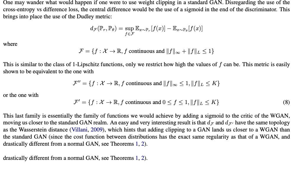
I find this interesting, though what certainly muddies the waters a bit is that there evidence to suggest that in practice a Lipschitz’d JS-GAN performs better than a Lipschitz’d WGAN:
- it seems to be the case in the spectral norm paper (though the comparisons between JS and WGAN actually used gradient penalty, not spectral norm);
- some peeps here and here posted issues on getting SN to work with WGAN, and even the author of the spectral norm paper had trouble himself;
- I vaguely recall achieving lower Inception scores on an old project that used a WGAN-SN.
Maybe it’s a mystery for now, but if it’s any consolation, theoretically both the regularised JSGAN and WGAN formulations are very similar and in practice you should just use JS-GAN, or even better, the hinge loss proposed in [#ref:sn]. Spectral normalisation has been in PyTorch for quite some time now, and it’s as simply as wrapping each linear and conv layer in your discriminator with torch.nn.utils.spectral_norm:
import torch
from torch import nn

# spec norm is built into pytorch, and it's very
# plug and play
from torch.nn.utils import spectral_norm as spec_norm

n_in = 10
n_out = 20

layer_l = spec_norm(nn.Linear(n_in, n_out))

layer_c = spec_norm(nn.Conv2d(n_in, n_out, kernel_size=3))
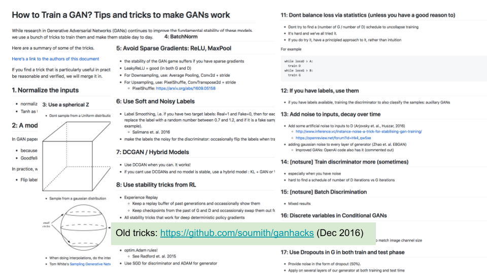
Prior to this work, these were many tricks that I saw on how to stabilise GAN training [#ref:gan_hacks]. While I don’t want to say that none of these have any utility anymore whatsoever, I have not had to use any of these. I feel however that any newcomers may stumble across such things and not realise that there are more straightforward ways to train GANs now.
Structuring the code cleanly
Clean code makes it easier to find bugs and reason about your code. Good abstractions are part of that. I like to have a train_on_batch(x) method, which performs a single gradient step over the batch x. Since GANs are a two-player game between \(G\) and \(D\) however, how do we structure the code? Which network should we train first?
Personally, I perform the gradient steps for the generator first, i.e., the \(G\) step. But it doesn’t matter which way you do it, as long as you’re careful as to how you’re handling the gradients. I’m going to be writing PyTorch-inspired pseudo-code (it’s using Python and PyTorch syntax but it’s not meant to be run per se, not unless you define a bunch of variables and implement the undefined methods I have written).
####################################################################
# This code is not meant to be executed -- it's simply pseudocode. #
####################################################################

REAL = 1
FAKE = 0

def train_on_batch(x_real):

    opt_g.zero_grad()
    opt_d.zero_grad()

    # --------------
    # First, train G
    # --------------

    z = sample_z(x_real.size(0))
    x_fake = G(z)
    g_loss = gan_loss( D(x_fake), REAL)
    # This backpropagates from the output of D, all the
    # way back into G.
    g_loss.backward()
    # G's gradient buffers are filled, we can perform
    # an optimisation step.
    opt_g.step()

    # ------------
    # Now, train D
    # ------------

    # IMPORTANT: D's grad buffers are filled because
    # of what we did above.
    opt_d.zero_grad()

    # x_fake.detach() not necessary here but it stops
    # grads from backpropagating into G. Even if that
    # did happen howwever, the start of `train_on_batch`
    # zeros both gradient buffers anyway, so it doesn't
    # matter.
    d_loss = gan_loss( D(x_fake.detach()), FAKE) + \
             gan_loss( D(x_real), REAL )
    d_loss.backward()
    opt_d.step()

    return g_loss.detach(), d_loss.detach()
What if you want to do it the other way around? Easy, though I find it’s a bit more confusing:
####################################################################
# This code is not meant to be executed -- it's simply pseudocode. #
####################################################################

REAL = 1
FAKE = 0

def train_on_batch(x_real):

    opt_g.zero_grad()
    opt_d.zero_grad()

    # ------------
    # Now, train D
    # ------------

    z = sample_z(x_real.size(0))
    x_fake = G(z)

    # Call `x_fake.detach()` because we don't want to
    # backpropagate gradients into G. If you didn't
    # use detach(), then when you call `g_loss.backward()`
    # later on you'd have to supply `retain_graph=True`.
    # Let's not do such confusing things...
    d_loss = gan_loss( D(x_fake.detach()), FAKE) + \
             gan_loss( D(x_real), REAL )
    d_loss.backward()
    opt_d.step()

    # ------------
    # Now, train G
    # ------------

    opt_d.zero_grad()

    g_loss = gan_loss( D(x_fake), REAL)
    # This backpropagates from the output of D, all the
    # way back into G.
    g_loss.backward()
    # G's gradient buffers are filled, we can perform
    # an optimisation step.
    opt_g.step()

    return g_loss.detach(), d_loss.detach()
You may see in some GAN implementations the use of backward(retain_graph=True) in order to be able to backprop through a particular graph more than once. For instance, in the code block directly before this you would have to use retain_graph=True if I didn’t detach() the tensor x_fake for the block that trains D. I have avoided such use of that here since I personally find it more confusing to think about.
Why have I defined a function gan_loss here? Because for certain GAN formulations (like JS-GAN), it helps a lot with readability. Rather than doing this, which can be relatively less readable and more error prone:
d_loss = -log(D(x_real)) - log(1-D(x_fake))
g_loss = -log(D(x_fake))
You could instead just write (at the expense of a few extra lines):
bce = nn.BCELoss()

# 1 = real, 0 = fake
ones = torch.ones((x_real.size(0), 1)).float()
zeros = torch.zeros_like(ones)

d_loss = bce( D(x_real), ones ) + bce( D(x_fake), zeros )
g_loss = bce( D(x_fake), ones )
Easy or common pitfalls to make
- Make sure that your generated samples are in the same range as your real data. For instance, if your real data is always in
[-1, 1]but your fake data is in[0, 1], that is something that the discriminator can pick up on to easily distinguish real from fake, and could result in degenerate training. My own rule of thumb is to always do non-fancy preprocessing on the real inputs: simply put it in the range[-1, 1]by performing(x-0.5)/0.5, and make the output of your generator functiontanh. When you want to visualise those images in matplotlib, simply denormalise by computingx*0.5 + 0.5. - If your generated images are not the same size (spatial dimension) as your real images, the discriminator can easily pick up on this and your generator loss will climb extremely high. This may seem like a no-brainer but I have made this mistake a few times. An example of this is MNIST: the default size of the images in
torchvision.datasets.MNISTis 28x28 but your generator architecture may generate 32x32 images, so in this case make sure you add atorchvision.transformthat resizes the MNIST digit to 32x32. - Batch norm can sometimes be unpredictable and result in wildly different generated images at training or test time (where in training time the batch statistics are computed over the minibatch, and at test time the moving averages are used). Usually I just use instance norm in place, of it. I’ve been bitten by batch norm’s intracacies too many times.
Plot your damn learning curves!
Most of the time when people come to me with GAN problems, they never come with graphs included and I usually have to ask for it. Sometimes I get no immediate response, and I wonder if it’s because they have to write code to do it, which certainly implies that their workflow isn’t very plotting-centric. Pessimistically it makes me wonder if the way most people debug things in deep learning is to just look at metrics flying down the terminal screen like this:
EPOCH: 001, TRAIN_D_LOSS: 0.4326436, TRAIN_G_LOSS: 1.352356, TIME: 435.353 SEC ...
EPOCH: 002, TRAIN_D_LOSS: 0.4521224, TRAIN_G_LOSS: 1.325623, TIME: 425.353 SEC ...
EPOCH: 003, TRAIN_D_LOSS: 0.4575744, TRAIN_G_LOSS: 1.657234, TIME: 422.533 SEC ...
EPOCH: 004, TRAIN_D_LOSS: 0.4025356, TRAIN_G_LOSS: 1.124543, TIME: 411.632 SEC ...
EPOCH: 005, TRAIN_D_LOSS: 0.4235636, TRAIN_G_LOSS: 1.457234, TIME: 450.353 SEC ...
...
...
...
(continue until your eyes get sore)
While our field does seem like the polar opposite of classical statistics (i.e. simple linear models, interpretability, etc.), we do have something in common with classical statistics, and that is in exploratory analysis. Just like classical statistics, deep learning should involve lots of exploratory analysis. Sure, that exploration isn’t going to be on 10,000-dimensional data (we can only see in three dimensions), but it will be on variables that your model is either optimising or measuring, which is extremely important to monitor if you want to know your network is training correctly. In our case, the losses are d_loss and g_loss, as defined in earlier pseudocode.
In Figure 3 I have illustrated these curves, left for a regular JS-GAN and on the right a spectrally normalised variant, SN-GAN.
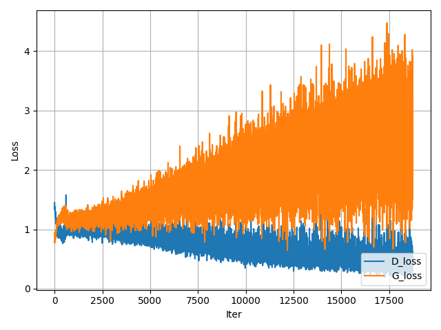
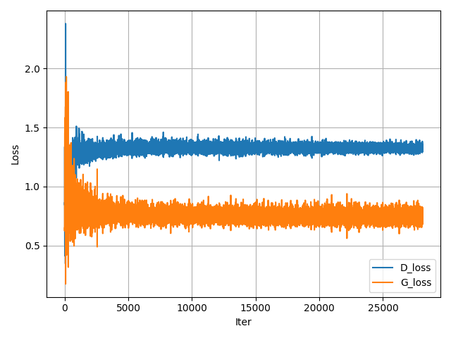
In my experience training SN-GAN (not JS-GAN), you want to be in a regime where the D loss is lower than the G loss but not by ‘too much’. For instance, if one loss is much larger or smaller than the other, this may be indicative of something problematic. For instance, if d_loss << g_loss (where << = significantly lower), this could mean your generator does not have enough capacity to model the data well and cannot compete well with the discriminator. Alternatively, if g_loss << d_loss, the discriminator may not be powerful enough, either. While you could use some sort of ‘balancing’ heuristic like roughly make both networks have the same # of learnable parameters, this is actually really crude. For instance, it’s expected \(G\) have way more parameters than \(D\) since it’s actually trying to model the data distribution (rather than simply distinguish between the two), so it doesn’t exactly set off alarm bells if your discriminator is only 5M parameters and your generator is 50M. Also, a 50M network with heavy weight decay does not have the same modeling capacity as one without it. Lastly, the issue certainly may not be in model complexity but rather the training dynamics. For example, if either network is really deep, are you making use of residual skip connections? If you’re concerned with vanishing gradients, you could also plot the average gradient norms here).
This is one of these things you will get a feel for after training lots of GANs. My best advice is to look at existing implementations of GANs on Github (ones that achieve good performance) and use their architectures as a base for your own work.
Because of Lipschitz, you don’t need to cripple your discriminator
Based on what I said about K-Lipschitz, it should certainly help (and not degrade gradients in any way) to give your discriminator a head start by training it for relatively more iterations than the generator. In other words, the better the discriminator is at distinguishing between real and fake, the better the signal that the generator can leverage from it. Note that as I mentioned earlier in this article, this logic did not make sense in the ‘pre-WGAN’ days because making the discriminator too good was detrimental to training.
In my own code, I simply keep track of the iteration number so that I can compute something like the following:
def train_on_batch(x, iter_, n_gen=5):
    # Generator
    ...
    ...
    if iter_ % n_gen == 0:
        g_loss.backward()
        opt_g.step()

    # Disc
    ...
    ...
    d_loss.backward()
    d_loss.step()
Where iter_ is the current gradient step iteration, and n_gen defines the interval between generator updates. In this case, since it’s 5, we can think of this as meaning that the discriminator is updated 5x as much as the generator.
Other people may do something like the following, preferring to leverage the data loader to perform such a thing:
def train(N):

    # number of discriminator iters per
    # generator iter
    n_dis = 5

    for iteration in range(N):

        for x_real in data_loader:
            # Update G
            train_on_batch_g(x_real)

        for _ in range(n_dis):
            for x_real in data_loader:
                # Update D
                train_on_batch_d(x_real)
Optimisers
The only optimiser I’ve really used for GANs is ADAM, and it seems like everyone else does as well. I don’t know why it works so well, but maybe it’s because all of our models have evolved over time to perform well on ADAM [#ref:adam_evolve], even if it may not necessarily be the right optimiser to always use.
[#ref:sn] presents a neat paper on various ADAM hps that they tried out, and which ones gave the best Inception scores:

As one can see here, for SN-GAN, option (C) performs best for CIFAR10 and option (B) for STL-10. Unfortunately however, as that graph shows, you can get wildly different optimal hps depending on what kind of GAN variant you are working with. In my own experience, I have found betas=(0, 0.9), lr=2e-4 to be a reasonable starting point.
Pesky hyperparameter: ADAM’s epsilon
ADAM’s default epsilon parameter in PyTorch is 1e-8, which may cause issues after a long period of training, such as your loss periodically exploding or increasing. See the StackOverflow post here as well as the Reddit comments here.
There may be some alternatives that alleviate this issue, such as Adamax. But I have not tried using it yet with GAN training.
Evaluation metrics
The two most commonly used metrics are Inception and FID, though there have been a whole host of other ones proposed as well. Unfortunately, these metrics can often be rather frustrating to use, and I will detail as many reasons as I can for this below.
Here are some things you should keep in mind about FID:
- Depending on how FID is calculated, it may only be appropriate to use it as a measure of underfitting, not overfitting. Looking at the code of pytorch-fid, which in turn is based on test, the pre-computed FID statistics for a particular dataset may be based on either the training set, the validation set, or both sets. For CIFAR10, it looks like it’s the training set. This means that if your generative model ‘cheated’ and simply memorised the training set, you’d get an FID of zero. I don’t know what % of GAN papers compute FID on train/valid/test but this seems like yet another confounding factor that makes reproducibility hard.
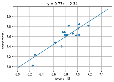
- Like Inception (see above), these scores are different depending on what pre-trained weights are used for the Inception network, which typically differ depending on whether the implementation is in PyTorch or TensorFlow. It seems like pytorch-fid now uses the same weights as the Inception network in TF, but I recall a few years back having to use a different set of weights for PyTorch with this code. I managed to dig up some old numbers where I evaluated various hyperparameters of a GAN I trained using both TF and PyTorch implementations, and got wildly different results (see Appendix).
There are other problems too. See ‘A note on the inception score’ [5] for a comprehensive critique of these scores.
Either way, you should be monitoring these metrics during training, as opposed to simply training the GAN for a fixed number of epochs and evaluating them afterwards. Think about this as being no different from training a classifier and monitoring its validation set accuracy during training: you want to know if image quality is improving over time, and you want to know if you’re able to stop training early when the FID/Inception plateaus or gets worse. Since these metrics can be expensive to compute, set up your code so that the metrics are computed every few epochs, so that you don’t completely bottleneck your training time.
Which is the best?
Ultimately, I feel like whatever evaluation metric you use really depends on what your downstream task is. If you just want to generate pretty images then sure, use something like FID or Inception. If however you are using GANs for something like data augmentation, then an appropriate metric would be training a classifier on that augmented data and seeing how well it performs on a held-out set.
While GANs are great in many aspects, one of their biggest downsides is not having a theoretically straightforward way of evaluating likelihoods. VAEs more or less give you this, by allowing you to compute a lower bound on \(p(x)\).
Conditioning on more than one noise variable
Sometimes you may want to train a more flexible generator, one that is able to be conditioned on more than one noise variable. For instance, rather than \(G(z)\) you may want \(G(z, c)\), where \(c \sim p(c)\) comes from some other prior distribution, e.g. a Categorical distribution. If you train the GAN, you will most likely find that it completely ignores one noise variable and uses the other.
In order to resolve this, you should turn to InfoGAN [#ref:infogan]. Put simply, the discriminator should have two additional output branches, one to predict both latent codes fed into the generator, and you should train the discriminator to be able to predict these codes from the generated image. In other words, we want to maximise the mutual information between the original codes input \((z, c)\) and the generated image \(G(z, c)\). One caveat however, we actually want to minimise such a loss with respect to both generator and discriminator; so this loss isn’t adversarial per se, but more like a ‘cooperative’ loss that both networks have to minimise. Here is some pseudo-code, assuming \(p(c)\) here is a Categorical distribution:
def train_on_batch(x):

  opt_d.zero_grad()
  opt_g.zero_grad()
  # or opt_all.zero_grad()

  c = sample_c(x.size(0))
  z = sample_z(x.size(0))

  # generator loss
  x_fake = G(z, c)
  ...
  ...
  # discriminator loss
  d_realfake, _, _ = D(x_fake)
  ...
  ...

  # `opt_all` wraps both the generator
  # and discriminator parameters, since we
  # we want to minimise the infogan loss
  # wrt to both networks.
  opt_all.zero_grad()
  # imagine D has three output layers: one
  # to determine real/fake, and the other two
  # for our noise variables.
  _, d_out_c, d_out_z = D(x_fake)
  z_loss = torch.mean((d_out_z-z)**2)
  # you could also use mean squared error here,
  # but i'm using the x-entropy to be more correct
  # about it, since p(c) is a multinomial distribution.
  # this means that `d_out_c` has been transformed with
  # the softmax nonlinearity.
  c_loss = categorical_crossentropy(d_out_c, c).mean()
  infogan_loss = z_loss + c_loss
  infogan_loss.backward()
  opt_all.step()
Resources
- [a]: PyTorch generative model collections. Figure 3’s JS-GAN was trained with this repo, spectral normalisation was added to the code by wrapping each linear and conv definition in
GAN.py. - [b]: Christian Cosgrove’s minimal HingeGAN + spectral norm implementation on CIFAR10. It was very useful to me when I started getting serious about GANs a few years ago.
Conclusion
If you think I’ve missed something or you’ve spotted an error, please let me know in the comments section at the bottom of this page or reach out to me on Twitter!
References
- [1]: https://colinraffel.com/blog/gans-and-divergence-minimization.html
- [2]: Arjovsky, M., Chintala, S., & Bottou, L. (2017, July). Wasserstein generative adversarial networks. In International conference on Machine Learning (pp. 214-223). PMLR.
- [3]: Gulrajani, I., Ahmed, F., Arjovsky, M., Dumoulin, V., & Courville, A. (2017). Improved training of Wasserstein GANs. arXiv preprint arXiv:1704.00028.
- [4]: https://github.com/soumith/ganhacks
- [5]: Barratt, S., & Sharma, R. (2018). A note on the inception score. arXiv preprint arXiv:1801.01973.
- [6]: Farnia, F., & Ozdaglar, A. (2020, November). Do GANs always have Nash equilibria?. In International Conference on Machine Learning (pp. 3029-3039). PMLR.
- [7]: https://parameterfree.com/2020/12/06/neural-network-maybe-evolved-to-make-adam-the-best-optimizer/
- [8]: Miyato, T., Kataoka, T., Koyama, M., & Yoshida, Y. (2018). Spectral normalization for generative adversarial networks. arXiv preprint arXiv:1802.05957.
- [9]: Chen, X., Duan, Y., Houthooft, R., Schulman, J., Sutskever, I., & Abbeel, P. (2016, December). InfoGAN: Interpretable representation learning by information maximizing generative adversarial nets. In Proceedings of the 30th International Conference on Neural Information Processing Systems (pp. 2180-2188).
Appendix
The relationship between PyTorch and TF Inception scores
import pandas as pd
import matplotlib.pyplot as plt
%matplotlib inline

df = pd.read_csv("./incep_tf_vs_pt.csv", names=["pytorch", "tensorflow"])
df
| pytorch | tensorflow | |
|---|---|---|
| 0 | 6.78 | 7.68 |
| 1 | 6.82 | 7.63 |
| 2 | 6.75 | 7.68 |
| 3 | 6.73 | 7.40 |
| 4 | 6.63 | 7.48 |
| 5 | 6.85 | 7.81 |
| 6 | 6.29 | 7.24 |
| 7 | 6.92 | 7.66 |
| 8 | 7.03 | 7.63 |
| 9 | 6.98 | 7.62 |
| 10 | 7.18 | 7.81 |
| 11 | 6.80 | 7.60 |
| 12 | 6.79 | 7.63 |
| 13 | 7.01 | 7.76 |
| 14 | 7.03 | 7.84 |
| 15 | 6.25 | 7.02 |
| 16 | 6.82 | 7.62 |
from sklearn import linear_model
import numpy as np
lm = linear_model.LinearRegression()

X = df['pytorch'].values.reshape(-1, 1)
y = df['tensorflow'].values.reshape(-1, 1)

lm.fit(X, y)

plt.scatter(X, y)
plt.ylabel('tensorflow IS')
plt.xlabel('pytorch IS')

xs = np.linspace(6, 7.5, num=100).reshape(-1, 1)
ys = lm.predict(xs)
plt.plot(xs, ys)
plt.grid()
lm_str = "y = %.2fx + %.2f" % (lm.coef_[0][0], lm.intercept_[0])
plt.title(lm_str)